
When you only want to add the numbers that meet a rule, the SUMIF function in Google Sheets does it in one step. Tell it what to look for and which numbers to total, and it adds only the matching rows.
This article covers five practical examples, including text matches, number thresholds, wildcards, and excluding a category. Each one uses a small dataset you can rebuild in a moment.
SUMIF Function Syntax in Google Sheets
Here is how the function is put together.
=SUMIF(range, criterion, [sum_range])
- range is the set of cells SUMIF checks against your condition.
- criterion is the test a cell must pass, such as “East”, “>100”, or “A*”.
- sum_range is optional. It holds the numbers to add. Leave it out and SUMIF totals the range it just tested.
When to Use SUMIF Function
SUMIF shines whenever a total needs a condition attached. A few common cases:
- Totaling sales for one region, one product, or one person.
- Adding only the values above or below a threshold.
- Summing amounts whose label starts with certain letters.
- Excluding a single category from a running total.
- Building a quick summary table without a pivot table.
Example 1: Sum Values That Match a Text Label
The core SUMIF job is totaling rows that match a word.
Below is the dataset. Column A lists regions, with East appearing several times, and column B holds the sales for each row.
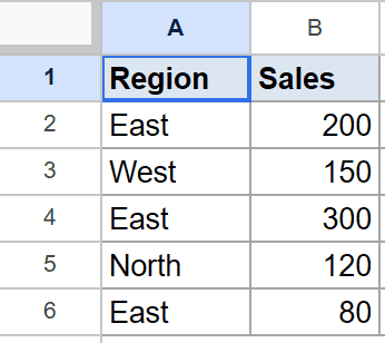
You want the total sales for the East region only.
Here is the formula:
=SUMIF(A2:A6, "East", B2:B6)
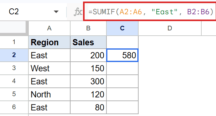
SUMIF checks column A for “East”, then adds the matching values from column B. The total comes to 580.
The three East rows are added together. Every other region is ignored.
Pro Tip: Text criteria are not case sensitive. “East”, “east”, and “EAST” all match the same rows.
Example 2: Sum Numbers Above a Threshold
Sometimes the column you test is also the column you want to total.
Below is the dataset. Column A lists products and column B holds the units sold for each.
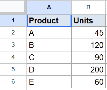
You want the total units for products that sold more than 100.
Here is the formula:
=SUMIF(B2:B6, ">100")
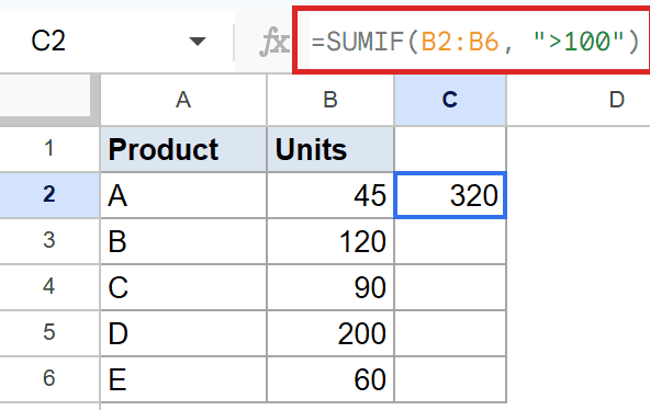
When the test range and the sum range are the same, you can skip the third argument. SUMIF tests column B and adds the same cells that pass.
Only the two values above 100 qualify, so the result is 320.
Example 3: Test One Column, Total a Different One
The range you check and the range you add do not have to be the same.
Below is the dataset. Column A holds salesperson names, column B holds their region, and column C holds the deal amount.
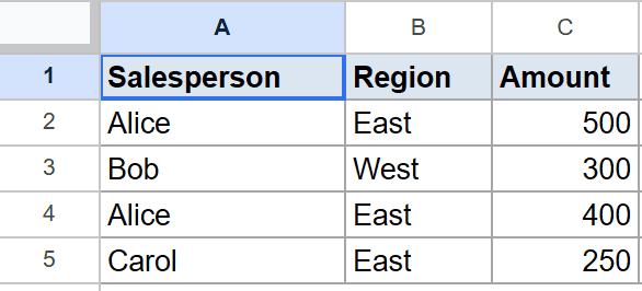
You want to total the amounts in column C, but only for rows where the region is East.
Here is the formula:
=SUMIF(B2:B5, "East", C2:C5)
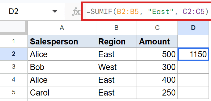
SUMIF tests column B for “East” and totals the matching cells from column C. The two columns stay separate.
The matching deals add up to 1150.
Pro Tip: The range and the sum_range should be the same height. Mismatched sizes can give you a wrong total without an obvious error.
Example 4: Sum Using a Wildcard Text Match
SUMIF understands wildcards, so you can match partial text.
Below is the dataset. Column A lists customer names and column B holds the amount each one spent.
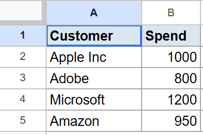
You want the total spend for every customer whose name starts with the letter A.
Here is the formula:
=SUMIF(A2:A5, "A*", B2:B5)
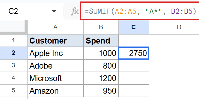
The asterisk stands for any run of characters. So “A*” matches any name that begins with A, no matter what follows.
Apple, Adobe, and Amazon all qualify while Microsoft is left out. The total is 2750.
Example 5: Sum Everything Except One Category
You can also total every row that does not match, using the not-equal operator.
Below is the dataset. Column A lists spending categories and column B holds the cost of each entry.
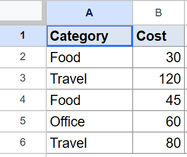
You want the total cost of everything that is not in the Food category.
Here is the formula:
=SUMIF(A2:A6, "<>Food", B2:B6)
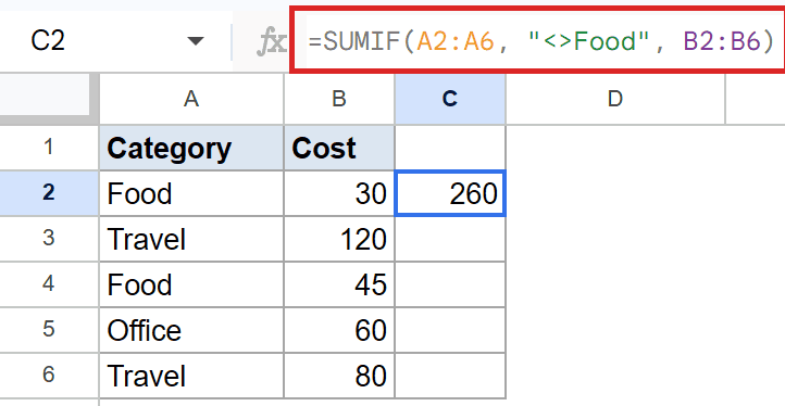
The “<>” operator means “not equal to”. So the criterion keeps every row whose category is anything other than Food.
The Travel and Office rows are added while both Food rows drop out. The result is 260.
Tips & Common Mistakes
- Wrap operators and text in quotes. Criteria like “>100”, “<>Food”, and “A*” must be inside double quotes, or the formula will not parse.
- For more than one condition, switch to SUMIFS. SUMIF handles a single test only. When you need region and month together, the SUMIFS function takes multiple criteria.
- Reference a cell instead of hardcoding. You can point the criterion at a cell, such as =SUMIF(A2:A6, E1, B2:B6), so changing E1 updates the total without editing the formula.
SUMIF turns a long list into a clean conditional total without a pivot table. Start with a simple text match, then move on to thresholds, wildcards, and exclusions as you need them.
When one condition is not enough, SUMIFS is the natural next step.
List of All Google Sheets Functions
Related Google Sheets Functions / Articles: