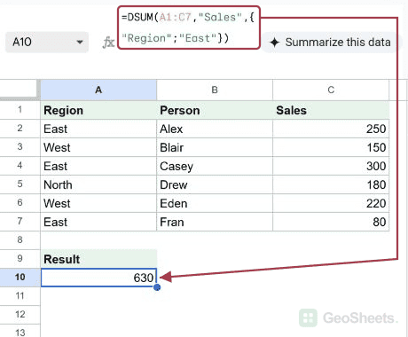
If you have a table-style range and you want to total one column for the rows that match some criteria, the DSUM function in Google Sheets does it in a single call.
It treats your range like a small database, looks at a separate criteria block to figure out which rows count, and sums the chosen column. In this article, I’ll show you how to use DSUM with a few practical examples.
DSUM Function Syntax in Google Sheets
Here is how the DSUM function is written:
=DSUM(database, field, criteria)
- database is the range that holds the table, including the header row. Every column needs a header in the top row.
- field is the column you want to total. You can pass the column header in quotes, like
"Sales", or its 1-based column position inside the database range, like3. - criteria is a small two-or-more-row range that tells DSUM which rows to include. The top row has column headers, the rows below hold the conditions.
The criteria range is the part that trips most beginners up. Spend a minute on the structure: column header on top, condition(s) underneath. Conditions on the same row are joined with AND. Conditions on separate rows are joined with OR.
When to Use DSUM Function
- Total a column from a table-style range using one or more criteria.
- Sum rows that match an OR condition (like East or West), which is awkward to express in SUMIFS.
- Build a small report area at the side of a table that updates as the criteria block changes.
- Combine comparison criteria like
>100with text criteria in the same query. - Reuse one criteria block for sibling functions like DCOUNT, DAVERAGE, and DMAX.
Example 1: Sum Sales for One Region
Let’s start with the simplest case, totaling sales for a single region.
Below is the dataset, with the database in A1:C7 holding Region, Salesperson, and Sales for six rows. The criteria block sits in E1:E2 with the header Region and the condition East.

You want a single number in G2 that totals the Sales column for every row where Region is East.
Here is the formula:
=DSUM(A1:C7,"Sales",E1:E2)

DSUM walks the database, checks each row against the criteria block, and adds up the Sales column for the rows that match. The three East rows hold 250, 300, and 80, so the total comes out to 630.
The field argument "Sales" tells DSUM which column to sum. The criteria range E1:E2 tells it which rows count.
Pro Tip: The criteria range header must match the database header exactly, character for character. A trailing space, a different case, or a typo will make DSUM come back empty with no warning. Copy the header directly from the database if you can.
Example 2: Sum Sales Above a Threshold
The criteria block isn’t just for equality. You can drop in a comparison expression and DSUM totals only the rows that pass it.
Below is the dataset, with the same database in A1:C7. The criteria block in E1:E2 uses the header Sales and the condition >200.

You want G2 to total only the Sales values that are greater than 200.
Here is the formula:
=DSUM(A1:C7,"Sales",E1:E2)

The criteria header is Sales, the same column we’re summing, and the condition >200 filters the rows. Three values clear that bar: 250, 300, and 220. They add up to 770.
Other comparison operators work the same way. Try >=100, <>0, or <200 in the criteria cell.
Pro Tip: Comparison criteria go in as text. The cell holds the literal string `>200`, not a formula. Type it in directly. Don’t start the cell with an `=` or Google Sheets will try to evaluate it.
Example 3: Sum With Two Criteria on the Same Row
When you put two conditions on the same row of the criteria block, DSUM treats them as an AND. A row has to match both to count.
Below is the dataset, with the database in A1:C7. The criteria block in E1:F2 has two headers, Region and Sales, with East and >100 directly below them.

You want H2 to total Sales for rows where Region is East AND Sales is greater than 100.
Here is the formula:
=DSUM(A1:C7,"Sales",E1:F2)

How this formula works:
- The criteria range now spans two columns, E and F.
- Row 2 has both conditions side by side, so DSUM applies them together as an AND.
- East rows over 100 are 250 and 300. The 80 row is East but fails the comparison, so it drops out.
The total comes to 550. Add a third column to the criteria block and you have a three-way AND. The pattern scales.
Example 4: Sum With Criteria Stacked on Separate Rows
Stack two conditions on separate rows of the same criteria column and DSUM joins them with OR. A row matches if it satisfies either one.
Below is the dataset, with the database in A1:C7. The criteria block in E1:E3 has the header Region in E1, then East stacked on top of West in E2 and E3.

You want G2 to total Sales for rows where Region is East OR Region is West.
Here is the formula:
=DSUM(A1:C7,"Sales",E1:E3)

How this formula works:
- The criteria range covers three rows, E1:E3. The header is in E1, the conditions in E2 and E3.
- Separate rows mean OR, so a database row matches if its Region is East or West.
- That picks up five rows out of six. North is the only one that drops.
Adding the matching sales gives 1000. This OR-on-stacked-rows pattern is the thing DSUM does that’s clumsy in SUMIF and SUMIFS.
Example 5: Use a Column Number for the Field
The middle argument of DSUM is the column to sum. You can pass it as a quoted header or as a 1-based column number inside the database. Both work.
Below is the dataset, with the database in A1:C7. The criteria block in E1:E2 filters Region to North.

You want G2 to total Sales for the North region, but instead of passing "Sales" as the field, pass 3 since Sales is the third column of the database.
Here is the formula:
=DSUM(A1:C7,3,E1:E2)

The 3 tells DSUM to look at the third column of the database range, which is Sales. There’s only one North row in the table, holding 180, so that’s the total.
The column-number form is handy when your header is long or has tricky characters. The quoted-header form is friendlier when someone else reads the formula. Use whichever fits.
Tips & Common Mistakes
- Criteria headers must match database headers. A trailing space, a different case, or a typo silently returns 0. If DSUM is giving you a zero you weren’t expecting, that’s the first thing to check.
- DSUM vs SUMIFS. SUMIFS is the modern default for multi-condition sums. It’s compact and doesn’t need a criteria block sitting on the sheet. DSUM still wins when you have OR conditions on the same column (the stacked-row trick) or when one criteria block needs to feed several D-functions at once. Pick the one that reads cleanly for the job.
- Comparison criteria are text strings. A condition like
>200lives in the cell as plain text, not as a formula. Don’t put an equals sign in front. If you want to reference a cell, use">"&H1so the operator and the cell value get joined into a text string.
DSUM is the function to reach for when you have a tidy table, a small criteria block, and a column you want to total. Point it at the database, name the field, and hand over the criteria range.
Single-row criteria join with AND, stacked rows join with OR, and the field can be a header in quotes or a column number. Once the criteria pattern clicks, the same shape transfers to DCOUNT, DAVERAGE, DMAX, and the rest of the D-functions.
List of All Google Sheets Functions
Related Google Sheets Functions / Articles: