If you want to find the inverse hyperbolic sine of a number in Google Sheets, the ASINH function does it in one step. You give it a value, and it returns the number whose hyperbolic sine equals that value.
In this article, I’ll show you how ASINH works, what makes it different from regular ASIN, and four short examples you can use right away.
ASINH Function Syntax in Google Sheets
The ASINH function takes a single input.
=ASINH(value)
- value is the number you want the inverse hyperbolic sine of. Any real number works, positive, negative, or zero.
One number in, one number out.
When to Use ASINH Function
Here are some situations where ASINH fits.
- Reversing a SINH result to recover the original value.
- Engineering and physics formulas built on hyperbolic functions.
- Statistics work, like the inverse hyperbolic sine transform for skewed data.
- Any math task where inverse hyperbolic functions show up.
Example 1: Inverse Hyperbolic Sine of a Column
Let’s start by running ASINH down a column of values.
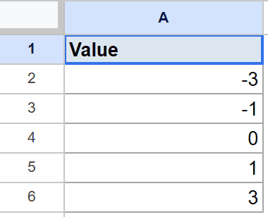
Below is the dataset with a single column of numbers, both negative and positive.
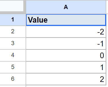
The goal is to get the inverse hyperbolic sine of each value in column A.
Here is the formula:
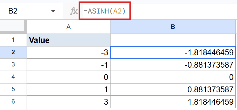
=ASINH(A2)
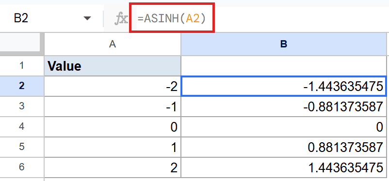
ASINH returns its answer in radians. Unlike ASIN, it accepts any real number, so there’s no domain limit to worry about. A value of 0 returns 0, 1 returns about 0.8814, and -2 returns about -1.4436.
Pro Tip: To run ASINH across a whole column in one formula, wrap it in ARRAYFORMULA: =ARRAYFORMULA(ASINH(A2:A6)). No filling down needed.
Example 2: Convert the Result to Degrees
Radians are fine for math, but a degree value is easier to picture.
Below is the dataset, a column of values to convert.
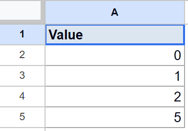
The goal is to read each ASINH result as an angle in degrees.
Here is the formula:
=DEGREES(ASINH(A2))
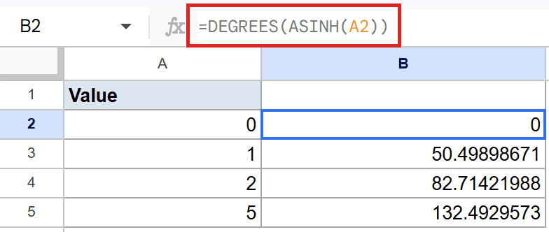
DEGREES converts the radian output from ASINH. So 0 still returns 0, 1 comes out near 50.5 degrees, and 5 lands around 132.49 degrees.
Example 3: ASINH Is Symmetric Around Zero
This example highlights a clean property of ASINH worth knowing.
Below is the dataset, matching negative and positive values around zero.
The goal is to compare the result of each negative input against its positive twin.
Here is the formula:
=ASINH(A2)
ASINH is symmetric around zero, meaning ASINH(-x) is the exact negative of ASINH(x). So 3 returns about 1.8184 and -3 returns about -1.8184. The value at 0 sits right in the middle at 0.
Example 4: Round the Result for Readability
The raw output runs to many decimal places, so rounding cleans up the column.
Below is the dataset, a short list of values.
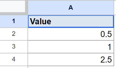
The goal is to trim each result to four decimal places.
Here is the formula:
=ROUND(ASINH(A2), 4)
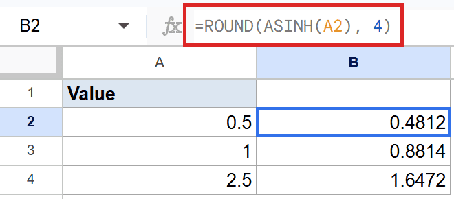
ROUND wraps the ASINH result and keeps four digits. So 0.5 returns 0.4812 and 2.5 returns 1.6472. Change the 4 to any number of decimal places you like.
Tips & Common Mistakes
- ASINH accepts any real number. There’s no domain limit like ASIN has, so negatives, zero, and large values all work without error.
- The result is in radians. Don’t read the raw output as degrees. Wrap it in DEGREES when you want a degree angle.
- Don’t confuse ASINH with ASIN. ASIN is the regular inverse sine, restricted to inputs from -1 to 1. ASINH is the hyperbolic version with no such limit.
ASINH is a one-argument function that returns the inverse hyperbolic sine of any real number, in radians. You saw how to run it down a column, convert it to degrees, confirm its symmetry around zero, and round the output.
With no domain limit to trip over, ASINH is one of the easier inverse functions to use.
List of All Google Sheets Functions
Related Google Sheets Functions / Articles: