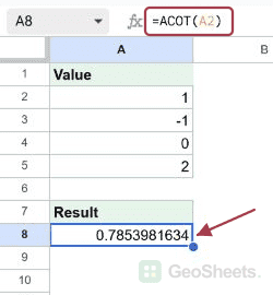
If you want to find the arccotangent of a number in Google Sheets, the ACOT function gives you the angle whose cotangent matches your value. You pass it one number and it returns the angle in radians.
In this article, I’ll show you how ACOT works, including one behavior with negative inputs that catches a lot of people off guard, plus four quick examples.
ACOT Function Syntax in Google Sheets
The ACOT function takes a single input.
=ACOT(value)
- value is the number you want the arccotangent of. Any real number works, including zero and negatives.
One number goes in, one angle comes out.
When to Use ACOT Function
Here are some common reasons to reach for ACOT.
- Recovering an angle from a known cotangent value.
- Geometry and trigonometry work where you start from a ratio and need the angle.
- Engineering or physics formulas built around inverse trig functions.
- Reversing a COT result to get back to the original angle.
Example 1: Arccotangent of a Column of Values
Let’s start by running ACOT down a list of positive numbers.
Below is the dataset with a single column of positive values.

The goal is to get the arccotangent of each value in column A.
Here is the formula:
=ACOT(A2)

ACOT returns the angle in radians. For positive inputs the result lands between 0 and about 1.5708. So 0.5 returns about 1.1071, and as the value grows the angle shrinks, with 5 returning roughly 0.1974.
Pro Tip: To run ACOT on a whole column in one shot, wrap it in ARRAYFORMULA: =ARRAYFORMULA(ACOT(A2:A5)). No need to fill down.
Example 2: Convert the Result to Degrees
Radians are great for math, but a degree value is easier to picture.
Below is the dataset, the same positive values from before.

The goal is to read each arccotangent as an angle in degrees.
Here is the formula:
=DEGREES(ACOT(A2))

The DEGREES function converts the radian output into degrees. A value of 1 returns exactly 45 degrees, 0.5 returns about 63.43 degrees, and 5 comes out near 11.31 degrees.
Example 3: How ACOT Treats Negative and Zero Inputs
This is the one to pay attention to, because ACOT does not behave the way the textbook arccotangent does.
Below is the dataset, a mix of negative values, zero, and positive values.

The goal is to see exactly what ACOT returns across the sign change at zero.
Here is the formula:
=ACOT(A2)

Google Sheets computes ACOT(x) as ATAN(1/x). At zero it returns about 1.5708, which is pi/2. Positive inputs return small positive angles.
Negative inputs are the gotcha. Instead of returning angles above pi/2, ACOT returns negative angles. So -1 returns about -0.7854 and -2 returns about -0.4636, not the values you’d get from the classic 0-to-pi definition.
Pro Tip: If you need the textbook arccotangent that maps negatives into the range above pi/2, add pi to the negative results: =IF(A2<0, ACOT(A2)+PI(), ACOT(A2)).
Example 4: Round the Result for Readability
The raw radian output runs to many decimals, so rounding tidies the column.
Below is the dataset, a short list of positive values.

The goal is to trim each result to four decimal places.
Here is the formula:
=ROUND(ACOT(A2), 4)

ROUND wraps the ACOT result and keeps four digits. So 1 returns 0.7854 and 3 returns 0.3218. Swap the 4 for however many decimals you want.
Tips & Common Mistakes
- Negative inputs return negative angles. Google Sheets uses ATAN(1/x), so ACOT(-1) is about -0.7854, not an angle above pi/2. Add PI() to negative results if you need the classic range.
- The result is in radians. Wrap ACOT in DEGREES whenever you want a degree value.
- Don’t confuse ACOT with ACOTH. ACOT is the arccotangent. ACOTH is the inverse hyperbolic cotangent, with a different domain and output.
ACOT is a one-argument function that returns the arccotangent of any number in radians. You saw how it works on positive values, how to convert to degrees, the negative-input quirk, and how to round.
The sign behavior is the thing to remember. Once you know ACOT follows ATAN(1/x), the rest is easy.
List of All Google Sheets Functions
Related Google Sheets Functions / Articles: