ACOSH Function in Google Sheets

If you want to find the inverse hyperbolic cosine of a number in Google Sheets, the ACOSH function does it in a single step. You give it a value, and it hands back the angle whose hyperbolic cosine equals that value.

In this article, I’ll walk you through how ACOSH works, where it fits, and four short examples you can copy straight into your own sheet.

ACOSH Function Syntax in Google Sheets

The ACOSH function takes just one input.

=ACOSH(value)
  • value is the number you want the inverse hyperbolic cosine of. It has to be 1 or greater.

That’s the whole signature. One number in, one number out.

When to Use ACOSH Function

Here are a few situations where ACOSH comes in handy.

  • Working through engineering or physics formulas that involve hyperbolic functions.
  • Reversing a COSH result to get back to the original value.
  • Modeling catenary curves, like the shape a hanging cable or chain makes.
  • Any math or stats work where inverse hyperbolic functions show up.

Example 1: Inverse Hyperbolic Cosine of a Column

Let’s start with the most basic use, running ACOSH down a list of numbers.

Below is the dataset with a single column of values, each one 1 or larger.

Google Sheets: Column A has header 'Value' and values 1, 1.5, 2, 5, 10.

The goal is to get the inverse hyperbolic cosine of each value in column A.

Here is the formula:

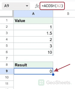
=ACOSH(A2)
Google Sheets shows =ACOSH(A2) formula in B2, producing 0, for input value 1.

ACOSH returns its answer in radians, not degrees. The first row, where the value is 1, returns 0. As the input grows, the result grows too, so 1.5 gives about 0.9624 and 10 gives about 2.9932.

Pro Tip: Instead of filling the formula down row by row, you can wrap it in ARRAYFORMULA to handle the whole column at once: =ARRAYFORMULA(ACOSH(A2:A6)). Same result, one formula.

Example 2: Convert the Result to Degrees

Radians are fine for math, but sometimes you want a degree value you can picture.

Below is the dataset, the same kind of value column with numbers of 1 or more.

Google Sheet showing ACOSH tutorial Example 2 dataset: "Value", 1, 2, 5, 10.

The goal is to read the ACOSH result as an angle in degrees instead of radians.

Here is the formula:

=DEGREES(ACOSH(A2))
Google Sheets: Formula `=DEGREES(ACOSH(A2))` highlighted in B2, showing result 0.

The DEGREES function takes the radian output from ACOSH and converts it. A value of 1 still returns 0, while 2 comes out to about 75.46 degrees and 10 lands near 171.5 degrees.

Example 3: ACOSH of 1 Returns Zero

This example shows what happens right at the edge of what ACOSH accepts.

Below is the dataset, starting at the smallest valid input and creeping up from there.

Google Sheet: "Value" header in A1, with data 1, 1.001, 1.5, 2 in cells below.

The goal is to see how the result behaves near the bottom of the allowed range.

Here is the formula:

=ACOSH(A2)
Google Sheets: B2 selected, formula bar shows =ACOSH(A2), cell B2 displays 0.

The smallest value ACOSH accepts is 1, and it returns 0 there. Just above it, 1.001 returns about 0.0447, so the curve climbs slowly at first. Anything below 1 would return an error instead of a number.

Pro Tip: If your data might contain values below 1, wrap ACOSH in an IF check like =IF(A2>=1, ACOSH(A2), “n/a”) so a stray number doesn’t break the column.

Example 4: Round the Result for Readability

ACOSH outputs a long decimal, so rounding makes the column easier to scan.

Below is the dataset, a short list of values to clean up.

Google Sheet: "Value" in A1, and dataset 1.5, 2, 3 in cells A2-A4.

The goal is to trim each result to four decimal places.

Here is the formula:

=ROUND(ACOSH(A2), 4)
Google Sheets example 4: cell B2 shows formula `=ROUND(ACOSH(A2), 4)`.

Here ROUND wraps the ACOSH result and keeps four digits after the decimal. So 1.5 returns 0.9624 and 3 returns 1.7627. Change the 4 to any number of places you prefer.

Tips & Common Mistakes

  • Inputs below 1 cause an error. ACOSH is only defined for values of 1 or higher, so anything smaller returns an error. Check your data first if it might dip below 1.
  • The result is in radians. Don’t read the raw output as degrees. Wrap it in DEGREES when you need a degree angle.
  • Don’t mix up ACOSH with ACOS. ACOS is the regular inverse cosine and accepts values from -1 to 1. ACOSH is the hyperbolic version with a totally different domain and output.

ACOSH is a one-argument function that gives you the inverse hyperbolic cosine of any value of 1 or more. You saw how to run it down a column, convert it to degrees, handle the edge at 1, and round the output.

Keep the domain rule in mind and the rest is straightforward.

List of All Google Sheets Functions

Related Google Sheets Functions / Articles: