If you want to multiply two columns row by row and then add up the results, the SUMPRODUCT function in Google Sheets does it in one step. It pairs up the values, multiplies each pair, and sums everything for you.
In this article, I’ll show you how SUMPRODUCT works, walk through four practical examples, and point out where it really shines.
SUMPRODUCT Function Syntax in Google Sheets
The SUMPRODUCT function takes one or more arrays of the same size.
=SUMPRODUCT(array1, [array2, ...])
- array1 is the first range or array of values.
- array2, … are optional extra ranges, each the same shape as the first.
SUMPRODUCT multiplies the arrays together position by position, then adds up all the products into a single number.
When to Use SUMPRODUCT Function
Here are a few times SUMPRODUCT comes in handy.
- Totaling order value when you have quantities in one column and prices in another.
- Building a weighted average without a helper column.
- Adding up numbers that meet a condition by multiplying with a true/false array.
- Counting rows that satisfy two or more conditions at once.
Example 1: Total Order Value from Quantity and Price
Let’s start with the classic use, turning quantities and prices into a grand total.
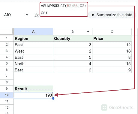
Below is the dataset, with a product in column A, a quantity in column B, and a unit price in column C.

The goal is to multiply each quantity by its price and add up all five line totals.
Here is the formula:
=SUMPRODUCT(B2:B6,C2:C6)

SUMPRODUCT multiplies each quantity by the price on the same row, then sums those five products. The result is 190, the full order value without needing a separate column for each line total.
Pro Tip: The arrays you pass must be the same size. If column B runs to row 6, column C has to run to row 6 as well, or you’ll get an error.
Example 2: Weighted Average Using SUMPRODUCT and SUM
SUMPRODUCT makes weighted averages easy.
Below is the dataset, with a subject in column A, a score in column B, and a weight in column C.

The goal is to find the average score where some subjects count more than others.
Here is the formula:
=SUMPRODUCT(B2:B6,C2:C6)/SUM(C2:C6)

How this formula works:
- SUMPRODUCT multiplies each score by its weight and adds those products together.
- SUM totals the weights so we know what to divide by.
- Dividing one by the other gives the weighted average, which here is 88.5.
Example 3: Conditional Sum with a Boolean Array
Here’s where SUMPRODUCT gets really useful.
Below is the dataset, with a region in column A and an amount in column B, with East repeating a few times.

The goal is to add up only the amounts where the region is East.
Here is the formula:
=SUMPRODUCT((A2:A7="East")*B2:B7)

How this formula works:
- The comparison
A2:A7="East"builds an array of TRUE and FALSE values, one per row. - Multiplying by column B turns each TRUE into 1 and each FALSE into 0, so non-East rows become zero.
- SUMPRODUCT then adds what’s left, giving 570 for the East rows.
Pro Tip: For a single straightforward condition, the SUMIF function is usually cleaner. SUMPRODUCT earns its keep when you start stacking multiple conditions together.
Example 4: Counting Rows with Two Conditions
You can multiply two true/false arrays to count rows that pass both tests.
Below is the dataset, the same region and amount table from the last example.

The goal is to count how many rows are both in the East region and above 100.
Here is the formula:
=SUMPRODUCT((A2:A7="East")*(B2:B7>100))

How this formula works:
- Each condition builds its own array of TRUE and FALSE values.
- Multiplying the two arrays gives a 1 only where both conditions are TRUE on the same row.
- SUMPRODUCT adds those 1s, so the count of East rows over 100 comes out to 3.
This counting trick is the same idea behind one approach to count cells with text in Google Sheets, where SUMPRODUCT tallies up a true/false array.
Tips & Common Mistakes
- All arrays must be the same shape. SUMPRODUCT pairs values by position, so a 5-row range and a 6-row range will throw an error. Keep your ranges aligned.
- Use the multiply trick for conditions. Multiplying comparison arrays inside SUMPRODUCT is how you handle multiple criteria. Each TRUE becomes 1 and each FALSE becomes 0.
- Reach for simpler tools when you can. For a plain conditional total, the SUMIFS function is easier to read. Save SUMPRODUCT for the cases those functions can’t handle cleanly.
SUMPRODUCT multiplies arrays together row by row and sums the results, all in a single formula. You saw it total order value, build a weighted average, sum with one condition, and count rows that pass two conditions.
Once the multiply-and-add pattern clicks, it becomes one of the most flexible tools in your kit.
List of All Google Sheets Functions
Related Google Sheets Functions / Articles: