
If you need an average where some values count more than others, the AVERAGE.WEIGHTED function in Google Sheets handles it in a single call.
You pass a range of values and a matching range of weights, and it returns the weighted mean. In this article, I’ll show you how to use AVERAGE.WEIGHTED with a few practical examples.
AVERAGE.WEIGHTED is a Google-Sheets-only function. Excel users typically reach for SUMPRODUCT(values,weights)/SUM(weights) to get the same result, which still works in Google Sheets too. AVERAGE.WEIGHTED is just the cleaner, purpose-built version.
AVERAGE.WEIGHTED Function Syntax in Google Sheets
Here is how the AVERAGE.WEIGHTED function is written:
=AVERAGE.WEIGHTED(values, weights, [additional values, additional weights, ...])
- values is the range of numbers you want to average.
- weights is the matching range of weights. Same shape and size as values.
- additional values, additional weights are optional extra pairs. You can pass as many value/weight pairs as you need; AVERAGE.WEIGHTED rolls them all into one result.
The function multiplies each value by its weight, sums the products, then divides by the sum of the weights. You don’t have to make the weights add up to 1 or 100. AVERAGE.WEIGHTED normalizes them on its own.
When to Use AVERAGE.WEIGHTED Function
- Calculate a course grade where homework, quizzes, and exams carry different weights.
- Find a portfolio return where each stock holds a different share of the total allocation.
- Average product ratings where some products have far more responses than others.
- Blend concentrations, prices, or scores across batches of different size.
- Combine values from multiple regions or groups into one overall figure.
Example 1: Weighted Course Grade Across Components
Let’s start with the most common use, a weighted course grade.
Below is the dataset, with Component, Score, and Weight as headers in row 1. Column A names the grade components, column B holds each component’s score out of 100, and column C holds the weight that component carries toward the final grade.
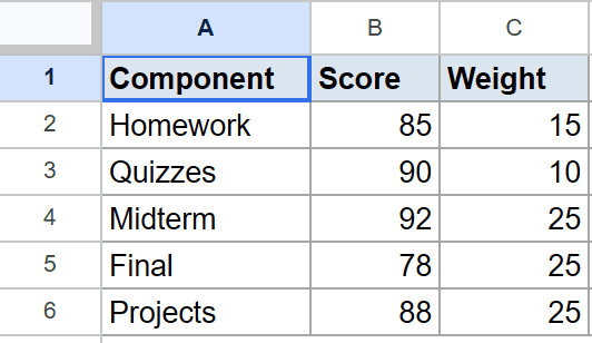
You want cell D2 to show the overall weighted grade across all five components.
Here is the formula:
=AVERAGE.WEIGHTED(B2:B6,C2:C6)
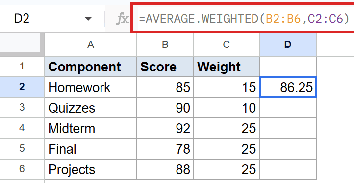
AVERAGE.WEIGHTED multiplies each score by its weight, adds those products, and divides by the total of the weights. The final result is 86.25.
A plain AVERAGE of column B would treat every component equally and land near 87. AVERAGE.WEIGHTED lets the heavier components pull the grade where it belongs.
Pro Tip: The weights don’t have to add up to 100, or to anything in particular. The function normalizes them automatically. Weights of 15, 10, 25, 25, 25 and weights of 0.15, 0.10, 0.25, 0.25, 0.25 give the same answer.
Example 2: Portfolio Return Weighted by Allocation
A textbook use case: figure out the overall return of a portfolio where each stock holds a different share of the money.
Below is the dataset, with Stock, Return %, and Allocation % as headers. Column A names the stocks, column B holds each stock’s return for the period, and column C holds the share of the portfolio that stock represents.
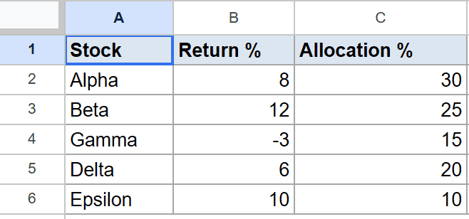
You want cell D2 to show the portfolio’s overall return, with each stock’s return weighted by its allocation.
Here is the formula:
=AVERAGE.WEIGHTED(B2:B6,C2:C6)
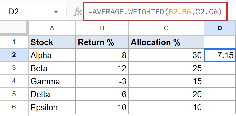
Same formula shape as before. The values are the returns, the weights are the allocations. The overall portfolio return is 7.15%.
Negative values work fine. The Gamma row carries a return of negative three, and AVERAGE.WEIGHTED handles it without complaint. It’s just another value to multiply by its weight.
Example 3: Average Rating Weighted by Response Count
When you’re averaging ratings across products with different sample sizes, treating every product as equally important hides the truth. Weight each rating by its response count and the big-sample products carry more pull.
Below is the dataset, with Product, Rating, and Responses as headers. Column A names the products, column B holds each product’s average rating, and column C holds the number of responses behind that rating.
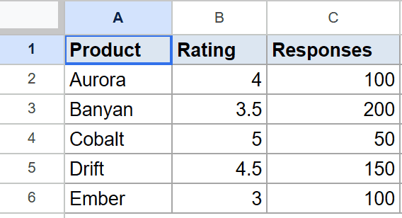
You want cell D2 to show the overall average rating, weighted by how many people responded for each product.
Here is the formula:
=AVERAGE.WEIGHTED(B2:B6,C2:C6)
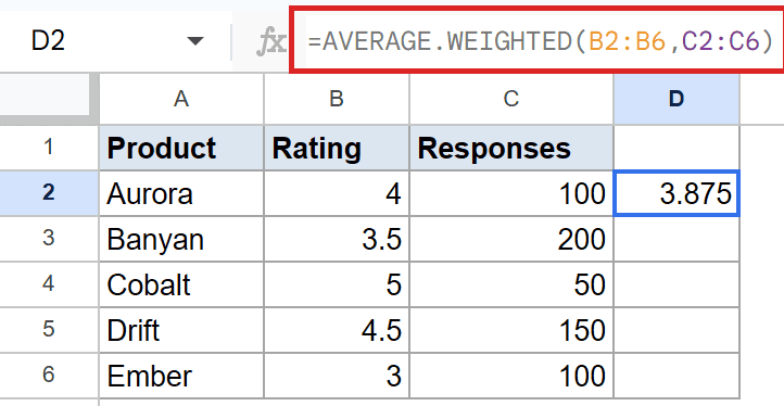
The Banyan product has 200 responses behind its 3.5 rating, so it pulls the overall figure down more than Cobalt’s 5-star rating with only 50 responses. The weighted average lands at 3.875.
A plain AVERAGE would land on four. The weighted version is closer to what customers actually see, since the products with more reviews are seen by more people.
Example 4: Blended Concentration Across Batches
When you mix batches of a liquid or a mixture, the resulting concentration depends on each batch’s volume. Bigger batches pull the blend toward their concentration.
Below is the dataset, with Batch, Concentration, and Volume as headers. Column A names the batches, column B holds the concentration of each batch, and column C holds the volume.
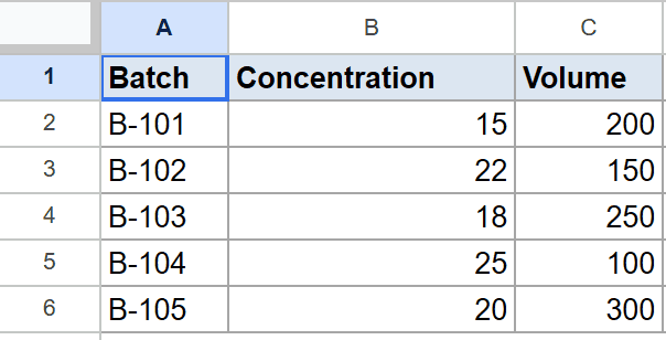
You want cell D2 to show the blended concentration after combining all five batches.
Here is the formula:
=AVERAGE.WEIGHTED(B2:B6,C2:C6)
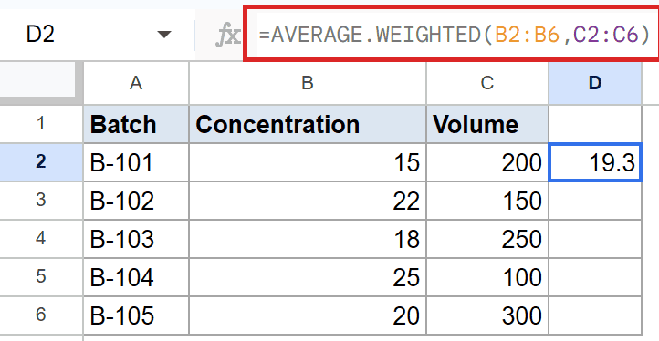
Each concentration is weighted by its batch volume. The 300-volume batch counts three times as much as the 100-volume batch, and so on. The blended concentration is 19.3.
Same pattern works for weighted prices across order sizes, weighted speeds across distance segments, and anything else where volume or size determines how much each input matters.
Example 5: Combine Two Regions Into One Weighted Average
When you have value and weight pairs in separate column groups, you don’t have to stack them. AVERAGE.WEIGHTED accepts more than one pair at a time.
Below is the dataset, with Product, East Price, East Units, West Price, and West Units as headers across columns A to E. Each row has a price and unit count for both the East and West regions.
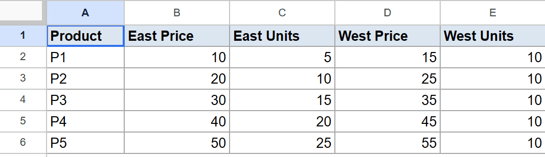
You want cell F2 to show one overall average price across both regions, with each price weighted by the units sold at that price.
Here is the formula:
=AVERAGE.WEIGHTED(B2:B6,C2:C6,D2:D6,E2:E6)
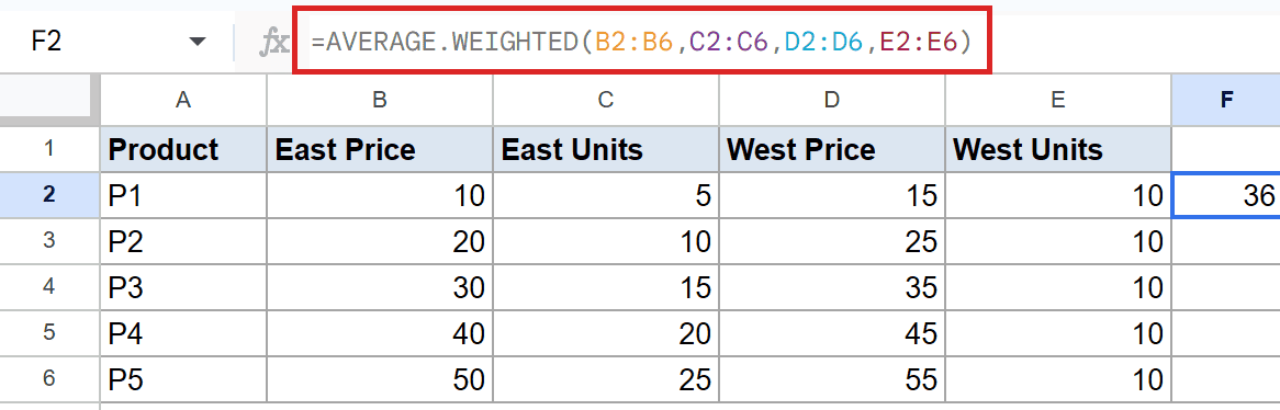
How this formula works:
- The first pair, B2:B6 and C2:C6, is the East prices and units.
- The second pair, D2:D6 and E2:E6, is the West prices and units.
- AVERAGE.WEIGHTED treats all four ranges as one big set of value/weight contributions and rolls them into a single weighted mean.
The combined weighted average price is 36. You could add a third region, a fourth, or any number more by stacking another value/weight pair on the end.
Pro Tip: In Excel, where AVERAGE.WEIGHTED doesn’t exist, the same calculation is `=SUMPRODUCT(B2:B6,C2:C6)/SUM(C2:C6)`. It works in Google Sheets too, so if you’re sharing a workbook with Excel users, that pattern travels safely. See the SUM function article for the SUM half of that expression.
Tips & Common Mistakes
- Values and weights must be the same shape. If you pass B2:B6 as values, weights have to be a five-row range too. A size mismatch returns a
#N/Aerror. Same shape applies for each extra pair. - Zero weights are fine, but they don’t all add up to zero. If every weight you pass is 0, AVERAGE.WEIGHTED returns
#DIV/0!because dividing by the total weight (which is 0) is undefined. A single zero weight inside a row of non-zero ones is harmless; that row just doesn’t contribute. - Negative weights work but rarely make sense. AVERAGE.WEIGHTED happily accepts negative weights and computes the result. Mathematically that’s a different beast from a weighted average; double-check the use case before you trust the number.
AVERAGE.WEIGHTED is the cleanest way to compute a weighted mean in Google Sheets. Hand it a values range and a weights range, optionally stack on more pairs, and you have your answer.
It shines for grades, portfolio returns, rating averages, and any other case where some inputs deserve more pull than others. The math is plain SUMPRODUCT divided by SUM; the function just saves you the typing.
List of All Google Sheets Functions
Related Google Sheets Functions / Articles: