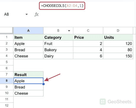
If you want to pull specific columns out of a range and stack them into a new array, the CHOOSECOLS function in Google Sheets does it in one shot. You hand it the source range and the column numbers you want, and it spills the chosen columns into the cells below.
In this article, I’ll show you how to use CHOOSECOLS to pick a single column, reorder columns, grab the last column with a negative index, and pair it with FILTER.
CHOOSECOLS Function Syntax in Google Sheets
The CHOOSECOLS function returns the columns you pick from an array, in the order you list them.
=CHOOSECOLS(array, col_num1, [col_num2, ...])
- array is the source range you’re picking columns from.
- col_num1 is the index of the first column to return. 1 is the leftmost column, 2 is the second column, and so on. Negative numbers count from the right, so -1 is the last column.
- col_num2, … are optional additional column indices. List them in the order you want the output columns to appear.
When to Use CHOOSECOLS Function
- Pull one or more specific columns out of a wider table.
- Reorder columns on the fly without touching the source data.
- Grab the rightmost column of a range without counting how many columns there are.
- Combine with FILTER, SORT, or QUERY to first trim rows and then pick columns.
- Build a clean output for a dashboard from a busy source table.
Example 1: Pick a Single Column From a Table
Let’s start with the simplest case, pulling one column out of a table.
Below is the dataset. Column A holds the order ID, column B has the customer name, column C is the region, and column D is the order total.
I want just the customer names, in their original order, returned as a spilling array.

Here is the formula:
=CHOOSECOLS(A2:D6, 2)

CHOOSECOLS looks at the range A2:D6, picks column number 2 (the customer column), and spills the five names down from E2. The other columns are ignored.
This works because CHOOSECOLS is a spilling function. You write the formula in one cell and the output fills the cells below automatically.
Example 2: Reorder Columns While You Pick Them
You can pick more than one column, and the order you list them is the order they come out in.
Below is the dataset. Column A has the product, column B has the SKU, column C has the price, and column D has the stock count.
I want the price first and the product name second, swapping their order from the source.

Here is the formula:
=CHOOSECOLS(A2:D5, 3, 1)

Column 3 (price) comes out first, then column 1 (product). CHOOSECOLS reads the indices left to right and builds the output in that same order.
This is handy when the source table is fixed and you need a different column order for a report or chart. No copy-paste, no helper columns.
Pro Tip: You can repeat the same index more than once. =CHOOSECOLS(A2:D5, 1, 1, 3) returns the product column twice followed by the price column, if you ever need a duplicate.
Example 3: Pick the Last Column With a Negative Index
Negative indices count back from the right side of the range.
Below is the dataset. Column A has the employee name, column B has the department, column C has the start year, and column D has the salary.
I want just the salary column, but I want to grab it by position from the right so the formula still works if I rearrange the source columns.

Here is the formula:
=CHOOSECOLS(A2:D5, -1)

The -1 tells CHOOSECOLS to take the last column of the range, which is the salary column. -2 would grab the second-to-last, and so on.
Negative indices are useful when you don’t know how wide the source range is, or when the rightmost column is always the one you care about. You can mix positive and negative indices in the same call too.
Example 4: Filter Rows Then Keep Only Two Columns
CHOOSECOLS pairs well with FILTER function, which trims rows down to the ones that match a rule. Wrap the filtered array inside CHOOSECOLS and you also get to pick which columns survive.
Below is the dataset. Column A has the item, column B has the category, column C has the price, and column D has the units sold.
I want only the rows where units sold is above 100, and from those rows I want just the item name and the price.

Here is the formula:
=CHOOSECOLS(FILTER(A2:D6, D2:D6>100), 1, 3)

How this formula works:
- FILTER first reduces A2:D6 down to the rows where column D is above 100. That keeps Apples, Cheese, Donut, and Eggs.
- CHOOSECOLS then takes that filtered array and pulls column 1 (item) and column 3 (price) from it.
- The output spills as a two-column array with the four surviving rows.
This pattern is where CHOOSECOLS really earns its keep. FILTER, SORT, or QUERY handles the row logic, and CHOOSECOLS does the column selection on top.
Tips & Common Mistakes
- Indices outside the range throw an error. If your source array is four columns wide and you ask for column 5, CHOOSECOLS returns a #VALUE! error. The same goes for a negative index that’s too far back, like -5 on a four-column array. Double-check the column count with COLUMNS function if you’re not sure.
- Leave room for the spill. CHOOSECOLS spills into the cells below and to the right of the formula cell. If any of those cells already have content, you’ll see a #REF! error. Clear the spill range or move the formula somewhere with empty space.
- CHOOSECOLS is the column twin of CHOOSEROWS. If you want to pick specific rows instead of columns, use CHOOSEROWS the same way. It also accepts negative indices to grab rows from the bottom.
CHOOSECOLS is the quickest way to slice the columns you want out of a bigger range. No helper columns, no copy-paste.
You’ve now seen it on a single column, reordered columns, a negative index, and inside a FILTER for a row-and-column trim in one formula.
List of All Google Sheets Functions
Related Google Sheets Functions / Articles: