
If you want the row number of a cell, the ROW function in Google Sheets hands it to you. It returns the absolute row number on the sheet, where the header sits in row 1 and your first data row is row 2.
In this article, I’ll walk you through five practical examples, including reading a cell’s own row, auto-numbering a list, banding alternate rows, and spilling a sequence with ARRAYFORMULA.
ROW Function Syntax in Google Sheets
ROW takes an optional cell reference and returns its row number.
=ROW([cell_reference])
cell_reference(optional): the cell or range you want the row number of. If you leave it out, ROW returns the row number of the cell the formula sits in.
When to Use ROW Function
- Get the absolute sheet row number of any cell.
- Auto-number a list so the numbering fixes itself when rows are added or deleted.
- Build alternating bands or groups with MOD for striped formatting or batching.
- Find the row number of a specific reference inside a larger formula.
- Generate a running sequence that spills down a column with ARRAYFORMULA.
Example 1: Return a cell’s own row number
Let’s start with the plainest case. You want each cell to report the row it lives on.
Below is the dataset with item names in column A and an empty row-number column B.
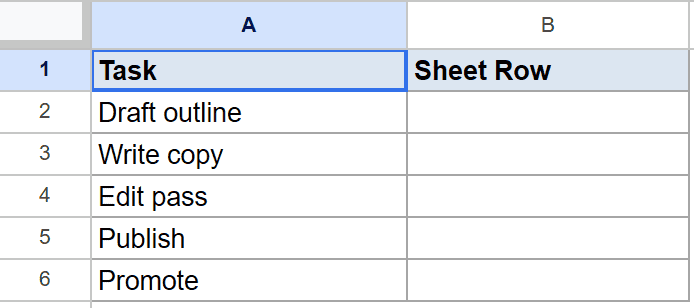
The goal is to show the absolute row number next to each item.
Here is the formula:
=ROW()
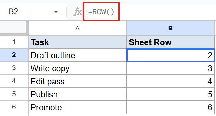
With no argument, ROW returns the row of the cell it sits in. In B2 that means it returns 2, not 1, because B2 is on the second row of the sheet. The header takes up row 1.
Filling down gives 3, 4, 5, and 6. The number always matches the sheet row, not the position within your data.
Example 2: Get the row number of a specific reference
ROW does not have to read its own cell. Pass it a reference and it returns that cell’s row instead.
Below is the dataset with text addresses in column A and an empty result column B.
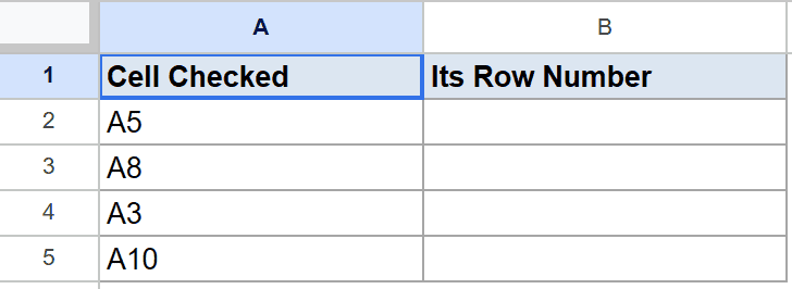
The goal is to read the address typed in column A and return its row number.
Here is the formula:
=ROW(INDIRECT(A2))
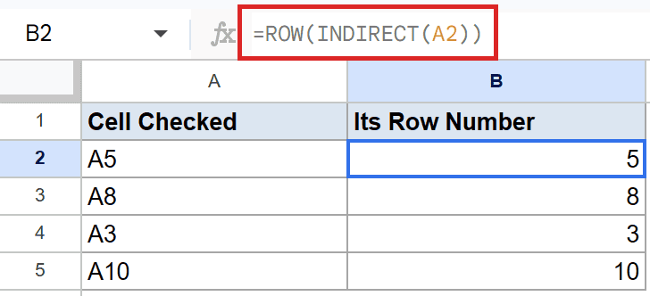
How this formula works:
- A2 holds a text address like
E5. The INDIRECT function turns that text into a real reference. - ROW then reports the row number of that reference, which is
5. - Filling down returns
8,3, and10for the addresses in the rows below.
Pro Tip: ROW pairs with the [COLUMN](https://geosheets.com/google-sheets-function/column/) function the same way. ROW gives you the vertical position and COLUMN gives you the horizontal one, which is handy when building addresses from parts.
Example 3: Auto-number a list
This is the most common reason people reach for ROW. You want a tidy 1, 2, 3 counter that ignores the header and repairs itself when rows change.
Below is the dataset with names in column A and an empty serial-number column B.
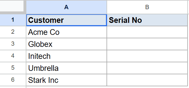
The goal is to number the data rows starting from 1, even though the first data row is sheet row 2.
Here is the formula:
=ROW()-1
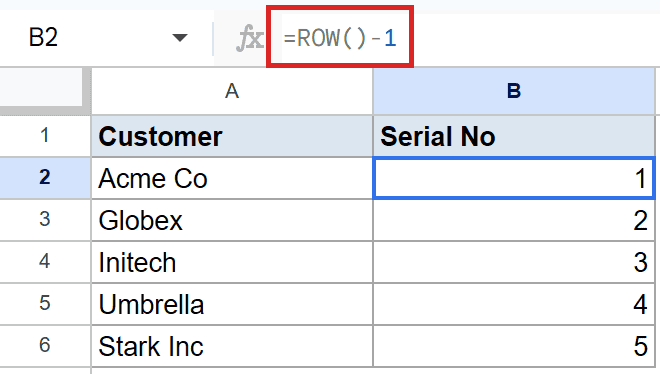
ROW in B2 returns 2, and subtracting 1 gives 1. B3 returns 3 minus 1, which is 2, and so on down to 5.
The big advantage over typing numbers by hand is that this fixes itself. Delete a row in the middle and the numbers below renumber on their own.
Example 4: Band alternate rows with MOD
ROW combined with MOD lets you tag every other row, which is the basis for striped formatting and alternating groups.
Below is the dataset with values in column A and an empty band column B.
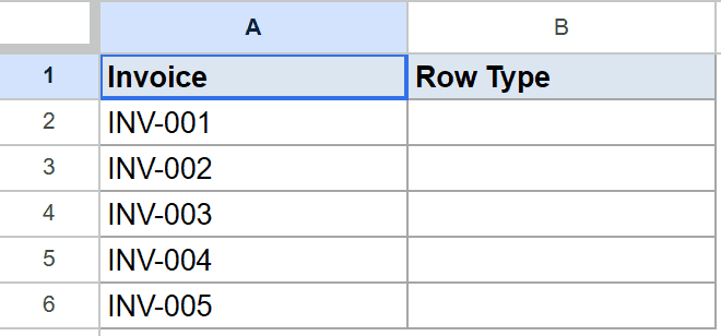
The goal is to mark each row as Even or Odd based on its sheet row number.
Here is the formula:
=IF(MOD(ROW(),2)=0,"Even","Odd")
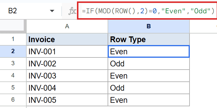
How this formula works:
MOD(ROW(),2)returns the remainder when the row number is divided by 2.- An even row gives a remainder of 0, so IF returns
Even. An odd row returnsOdd. - B2 sits on row 2, so it returns
Even. B3 returnsOdd, then the pattern alternates down the column.
Pro Tip: The same MOD(ROW(),N) trick groups rows in batches. Use 3 instead of 2 to tag every third row, which is useful for splitting data into repeating sets.
Example 5: Spill a sequence with ARRAYFORMULA
This example builds a running sequence that fills the whole column at once instead of being copied cell by cell.
Below is the dataset with labels in column A and an empty sequence column B.
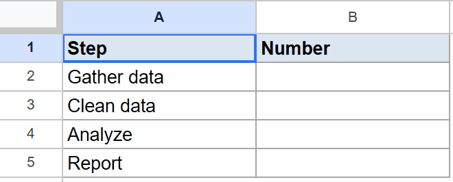
The goal is to number the four data rows from 1 with a single formula that spills down.
Here is the formula:
=ARRAYFORMULA(ROW(A2:A5)-ROW(A2)+1)
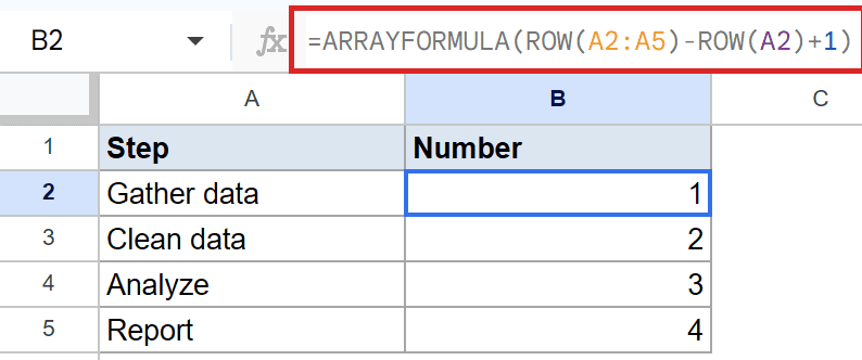
How this formula works:
ROW(A2:A5)returns the row numbers2, 3, 4, 5as an array.- Subtracting
ROW(A2), which is 2, and adding 1 shifts the sequence to start at 1. - ARRAYFORMULA spills the result into the four cells, giving
1,2,3, and4.
Only B2 holds the formula here. The other three values spill from it, so clicking B3 shows an empty formula bar.
Tips & Common Mistakes
- ROW returns the sheet row, not the data position. In B2 it returns 2, not 1, because row 1 is the header. Subtract the offset (usually
ROW()-1) when you want numbering that starts at 1. - ROW() with no argument is the cell it sits in. People expect
=ROW()in B2 to mean row 1 of the data. It means sheet row 2. Pass an explicit reference likeROW(A5)when you want a fixed row. - Don’t confuse ROW with the ROWS function. ROW returns a position. ROWS counts how many rows are in a range.
=ROW(A2:A5)returns 2, while=ROWS(A2:A5)returns 4.
ROW is one of those small functions that quietly powers a lot of useful patterns. Once you know the header sits in row 1 and your first data row is row 2, auto-numbering, banding, and sequence building all fall into place. It works hand in hand with the COLUMN function and the ADDRESS function when you need to locate or assemble cell positions.
List of All Google Sheets Functions
Related Google Sheets Functions / Articles: