
GETPIVOTDATA retrieves a summarized value by its pivot-table field and item names. Use it to keep a dashboard lookup tied to a category when pivot rows reorder.
GETPIVOTDATA function syntax
=GETPIVOTDATA(value_name, any_pivot_table_cell, [field1, item1, ...])- value_name: summarized value label, such as “SUM of Sales”. Use the exact displayed label when multiple value fields exist.
- any_pivot_table_cell: a cell inside the native pivot table. Its top-left corner is usually the safest anchor.
- field and item arguments come in pairs, such as “Region”,”East”. Add another pair for a second grouping.
- The requested value must be represented in the pivot table. A plain table is not a pivot table.
Set up the example data
Enter this dataset starting in A1. The first row contains headings. Keep the result area separate from the source table.
| Region | Quarter | Sales |
|---|---|---|
| East | Q1 | 1000 |
| East | Q1 | 1200 |
| East | Q2 | 1100 |
| West | Q1 | 800 |
| West | Q2 | 1500 |
| North | Q1 | 700 |
| North | Q2 | 900 |
Retrieve the pivot grand total
Create a pivot from A1:C8 at A12. Set Rows to Region, Columns to Quarter, and Values to Sales summarized by SUM. Keep row and column totals enabled. Enter this formula in A20.
=GETPIVOTDATA("SUM of Sales",A12)Result: 7200.
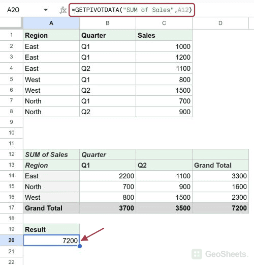
To total source rows without a pivot, use SUMIFS. QUERY can create a grouped summary directly from source data.
Retrieve one region total
Add the Region field and East item as a pair. The pivot contains three East orders: 1,000, 1,200 and 1,100. Their combined total is returned.
=GETPIVOTDATA("SUM of Sales",$A$12,"Region","East")Result: 3300.
Retrieve a value by region and quarter
The first pair selects West; the second selects Q2. Both field names refer to the grouping columns in the source data.
=GETPIVOTDATA("SUM of Sales",$A$12,"Region","West","Quarter","Q2")Result: 1500.
Read a count alongside a sum
Create a second pivot at J1 using the same source. Add Region to Rows and Sales twice to Values: one SUM and one COUNTA. Use the exact value label to retrieve the East order count.
=GETPIVOTDATA("COUNTA of Sales",$J$1,"Region","East")Result: 3.
Use an input cell for the region
Type North into F20. This formula reads the region from that cell, allowing you to switch the requested category without editing the formula.
=GETPIVOTDATA("SUM of Sales",$A$12,"Region",F20)Result: 1600.
Handle a missing pivot item
South does not appear in this pivot. The formula returns #REF! instead of zero, so a missing item is distinguishable from a genuine zero total.
=GETPIVOTDATA("SUM of Sales",$A$12,"Region","South")Result: #REF!.
Use a custom value heading
Create a region-only SUM pivot at J20 and rename its value heading Revenue. Use that displayed heading in GETPIVOTDATA, following Google guidance.
=GETPIVOTDATA("Revenue",$J$20,"Region","East")Result: 3300.
Other Google Sheets articles you may also like