If you want to round a number to the nearest multiple of something other than a power of ten, the MROUND function in Google Sheets is the one you want. It snaps any value to the nearest multiple of the factor you choose.
In this article, I’ll show you MROUND in action with five examples, from rounding prices to a quarter, to time blocks, to case-pack inventory and budget tiers.
MROUND Function Syntax in Google Sheets
Here is how you write the MROUND function.
=MROUND(value, factor)
- value – the number you want to round.
- factor – the multiple you want to round to. The value and factor must have the same sign, or one must be zero.
MROUND rounds to the nearest multiple. If the value sits exactly halfway between two multiples, it rounds away from zero.
When to Use MROUND Function
- Snapping prices to the nearest quarter, dime, or other denomination for cash handling.
- Rounding time durations to the nearest 5, 10, or 15 minute block for cleaner reports.
- Aligning inventory counts to case-pack sizes like 6, 12, or 24.
- Rounding large dollar amounts to a tidy budget boundary like $100 or $500.
Example 1: Round prices to the nearest $0.25
A classic use of MROUND is cash-handling rounding.
Below is the dataset, raw prices in column A and an empty Rounded column in B.
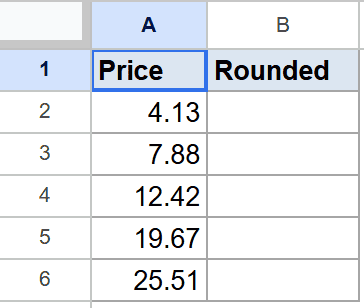
The goal is to snap each price to the nearest quarter dollar.
Here is the formula:
=MROUND(A2, 0.25)
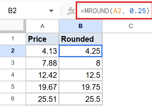
Each price rounds to its closest multiple of 0.25. 4.13 becomes 4.25, 7.88 becomes 8.00, 12.42 becomes 12.50, and so on down the column.
Example 2: Round meeting durations to nearest 15 minutes
Time tracking is another natural fit for MROUND.
Below is the dataset, raw minute counts in column A.
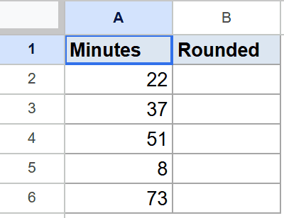
The goal is to snap each duration to the nearest 15-minute block.
Here is the formula:
=MROUND(A2, 15)
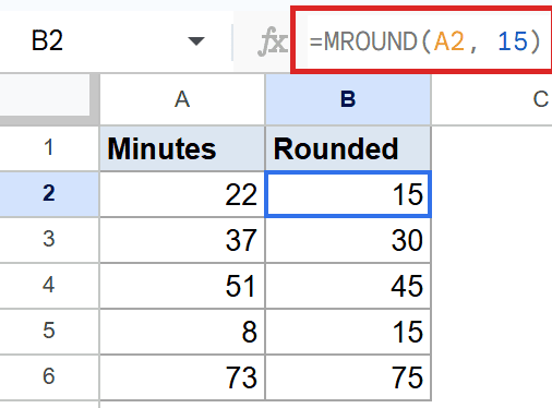
22 minutes lands at 15, 37 at 30, 51 at 45, and 73 at 75. The function picks whichever multiple of 15 is closest, no matter the direction.
Pro Tip: If you always want to round up, use CEILING instead of MROUND. If you always want to round down, use FLOOR. MROUND only picks the nearest multiple, in either direction.
Example 3: Round inventory counts to case-pack of 12
For ordering, you often want quantities that line up with case packs.
Below is the dataset, raw units-needed counts in column A.
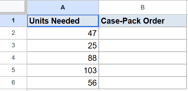
The goal is to round each count to the nearest multiple of 12, the case-pack size.
Here is the formula:
=MROUND(A2, 12)
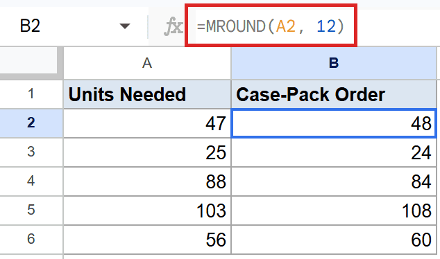
47 snaps down to 48, 25 snaps down to 24, 88 to 84, and 103 to 108. Each result is a whole number of cases.
Example 4: Round budget figures to nearest $500
For high-level budget reports, you usually want round numbers, not pennies.
Below is the dataset, amounts in column A ranging from a thousand to over twelve thousand.
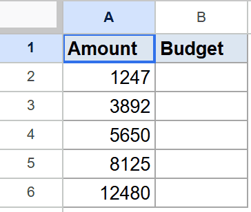
The goal is to snap each amount to the nearest $500.
Here is the formula:
=MROUND(A2, 500)
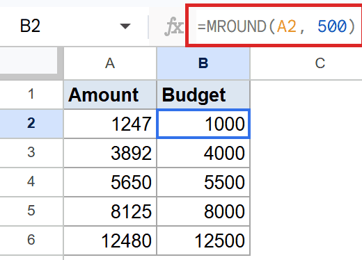
1247 rounds down to 1000, 3892 up to 4000, 5650 down to 5500, and 12480 up to 12500. Budget summaries become much easier to read.
Example 5: Round measurements to nearest 0.1
The factor can be a small decimal too.
Below is the dataset, sensor readings with two decimals in column A.
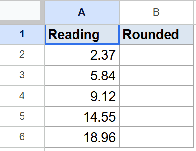
The goal is to round each reading to one decimal place.
Here is the formula:
=MROUND(A2, 0.1)
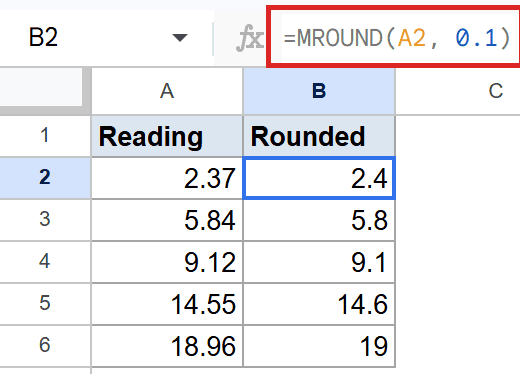
2.37 becomes 2.4, 5.84 becomes 5.8, 14.55 becomes 14.6, and 18.96 becomes 19. Same lesson as Example 1, just with a tighter factor.
Pro Tip: For plain decimal rounding (1, 2, or 3 decimal places), ROUND is usually quicker than MROUND. Reach for MROUND when the multiple isn’t a power of ten.
Tips & Common Mistakes
- Signs must match – if the value is negative, the factor has to be negative too, or zero. Mixing signs (like
=MROUND(-5, 2)) returns a #NUM error. - Halfway values round away from zero –
=MROUND(7.5, 5)returns 10, not 5. If you need banker’s rounding or always-up, use ROUND or CEILING instead. - A factor of zero returns zero –
=MROUND(50, 0)gives 0, not the original value. Make sure your factor cell isn’t blank or holding a stray zero.
MROUND is a small function that quietly cleans up a lot of business reporting. Once you stop reaching for ROUND for everything and start using the right rounding factor, prices, time blocks, and order quantities all line up the way you want them to.
List of All Google Sheets Functions
Related Google Sheets Functions / Articles: