If you want to cut a number down to a set number of decimal places in Google Sheets, the ROUND function is what you reach for. You tell it how many digits to keep and it rounds the rest away using normal rounding rules.
In this article, I’ll walk through how ROUND works with decimals, whole numbers, negative places, and a real pricing calculation.
ROUND Function Syntax in Google Sheets
The ROUND function rounds a number to a specified number of digits.
=ROUND(value, [places])
- value is the number you want to round.
- places is optional. It’s how many decimal places to keep. Leave it out or set it to 0 to round to the nearest whole number. A negative value rounds to the left of the decimal point.
ROUND uses standard rounding: 0.5 and above rounds up, below 0.5 rounds down.
When to Use ROUND Function
- Trimming long decimals down to two places for currency or percentages.
- Rounding a calculated value to the nearest whole number.
- Rounding to the nearest ten, hundred, or thousand with negative places.
- Cleaning up the output of another formula before it goes into a report.
- Making sure totals add up the way people expect, without trailing decimals.
Example 1: Round to Two Decimal Places
Let’s start with the most common use, keeping two decimals.
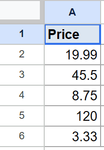
Below is the dataset, a single column of numbers with long decimals in A2 to A6.
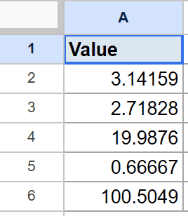
I want each number trimmed to two decimal places in column B.
Here is the formula:
=ROUND(A2, 2)
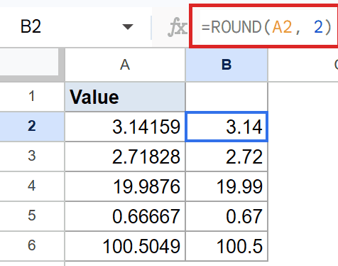
ROUND keeps two digits after the decimal point and rounds the third digit. So a value like 3.14159 becomes 3.14, and 19.987 rounds up to 19.99.
Pro Tip: ROUND changes the stored value, not just how it looks. If you only want a number to display with two decimals but keep its full precision underneath, use Format and number formatting instead.
Example 2: Round to the Nearest Whole Number
If you leave places at zero, ROUND snaps each number to the nearest integer.
Below is the dataset, a single column of decimal numbers in A2 to A6.
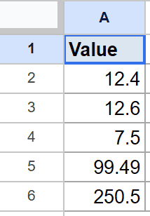
I want each number rounded to the nearest whole number in column B.
Here is the formula:
=ROUND(A2, 0)
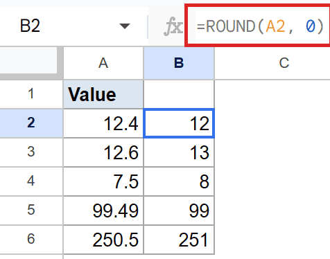
With places set to 0, ROUND looks at the first decimal to decide direction. A value of 12.4 rounds down to 12, while 12.5 would round up. The result for the first row is 12.
Example 3: Round to the Nearest Ten
A negative places value rounds to the left of the decimal point, which is handy for tidy round numbers.
Below is the dataset, a single column of three-digit numbers in A2 to A6.
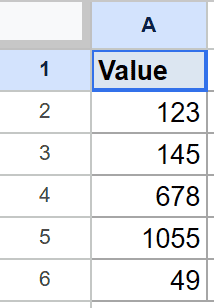
I want each number rounded to the nearest ten in column B.
Here is the formula:
=ROUND(A2, -1)
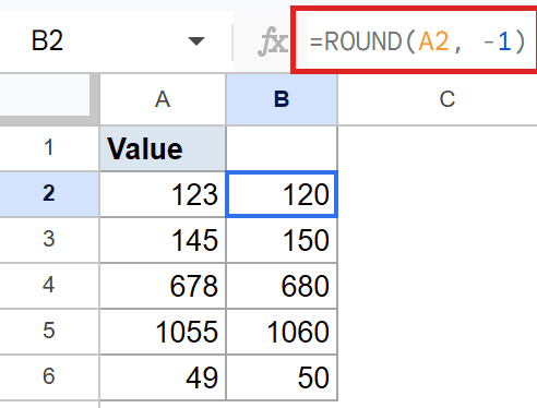
How this formula works:
- Places of -1 tells ROUND to round at the tens position.
- It looks at the ones digit to pick the direction.
- So 124 rounds down to 120, and 145 rounds up to 150. Use -2 for the nearest hundred and -3 for the nearest thousand.
Example 4: Rounding Negative Numbers
ROUND handles negative numbers by rounding away from zero on the halfway point, so it’s worth seeing in action.
Below is the dataset, a single column of small positive and negative decimals in A2 to A6.
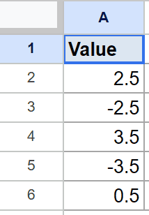
I want each value rounded to the nearest whole number in column B.
Here is the formula:
=ROUND(A2, 0)
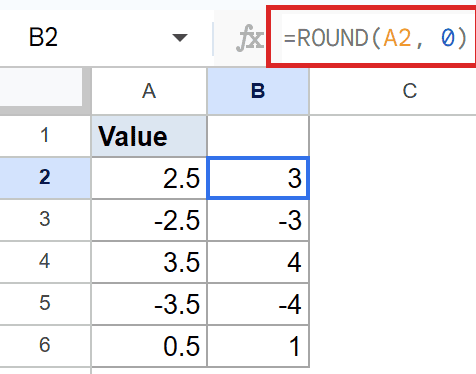
ROUND looks at the size of the number, then keeps the sign, much like the ABS function works on magnitude before anything else. A value of 2.5 rounds to 3, and -2.5 rounds to -3. The first row here rounds to 3.
Pro Tip: If you always want to round toward zero or always away from it regardless of the halfway rule, look at ROUNDDOWN and ROUNDUP. They ignore the 0.5 cutoff and force the direction.
Example 5: Round a Calculated Price
ROUND really earns its place when it wraps another calculation. Here we add tax and round to cents in one formula.
Below is the dataset, a single column of pre-tax prices in A2 to A6.
I want each price increased by 8 percent tax and rounded to two decimal places in column B.
Here is the formula:
=ROUND(A2*1.08, 2)
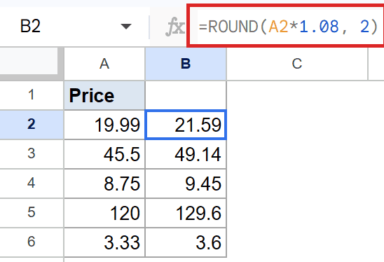
The multiplication happens first, then ROUND trims the result to two decimals so you get a clean price. For the first row, the formula returns 21.59 instead of a messy trailing decimal.
Tips & Common Mistakes
- ROUND changes the value, formatting doesn’t. Number formatting only changes what you see. ROUND changes the actual stored number, which matters when later formulas use the cell.
- Negative places round to the left. It’s easy to forget that -1 means tens, -2 means hundreds, and so on. A positive number keeps decimals, a negative one drops whole-number digits.
- Don’t confuse ROUND with ROUNDUP and ROUNDDOWN. ROUND follows the 0.5 rule. If you need to always push up or always push down, those two functions are the ones you want. To round up to a tidy multiple instead of a decimal place, the CEILING function is the better fit.
That’s ROUND in Google Sheets, from simple decimals to negative places and rounded calculations.
Once you’ve got the places argument figured out, rounding currency, percentages, and totals becomes second nature.
List of All Google Sheets Functions
Related Google Sheets Functions / Articles: