If you want to round numbers up so nothing ever gets rounded down, the ROUNDUP function in Google Sheets is what you need. It always pushes a number away from zero to the next step, which is handy when you can’t afford to fall short.
In this article, I’ll show you how ROUNDUP works with four practical examples.
ROUNDUP Function Syntax in Google Sheets
Here is how the ROUNDUP function is written:
=ROUNDUP(value, [places])
- value is the number you want to round up.
- places is optional. It sets how many decimal places to keep. Use 0 (the default) for whole numbers, a positive number for decimals, or a negative number to round up to tens, hundreds, and beyond.
The key thing to remember is that ROUNDUP always rounds away from zero. Even a value like 2.1 gets pushed up to 3, never down to 2.
When to Use ROUNDUP Function
- Rounding prices or totals up so you never undercharge.
- Working out how many boxes, pages, or batches you need with no leftover.
- Forcing decimals up to the next cent for billing.
- Rounding figures up to a clean ten or hundred for planning.
- Any time rounding down would leave you short.
Example 1: Round Up to a Whole Number
Let’s start with the simplest case, rounding decimals up to whole numbers.
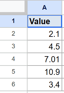
Below is the dataset. Column A holds a single list of decimal values in A2 to A6.
I want to round each value up to the next whole number in column B.
Here is the formula:
=ROUNDUP(A2, 0)
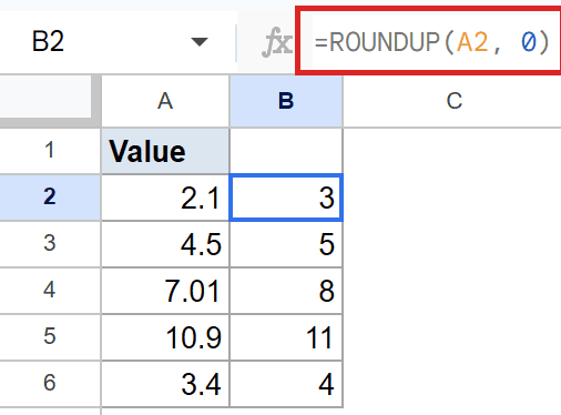
For the first value, 2.1, the formula returns 3. Notice that even 4.5 rounds up to 5 rather than staying at 4. ROUNDUP doesn’t care whether the decimal is above or below the halfway point, it always goes up.
I filled this formula down column B so each row rounds its own value. The 0 in the second slot means no decimal places, so you get whole numbers.
Pro Tip: This is the big difference between ROUNDUP and ROUND. ROUND follows normal rounding rules (2.1 goes to 2), while ROUNDUP always pushes up (2.1 goes to 3). ROUNDDOWN does the opposite and always pushes toward zero.
Example 2: Round Up to Two Decimal Places
You can keep decimal places instead of going all the way to whole numbers.
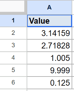
Below is the dataset. Column A holds values with several digits after the decimal point.
I want to round each one up to two decimal places, like rounding up to the nearest cent.
Here is the formula:
=ROUNDUP(A2, 2)
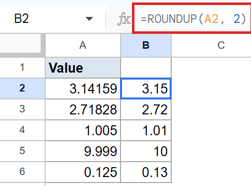
For 3.14159, the formula gives 3.15. The places argument is now 2, so it keeps two digits after the decimal and rounds that second digit up.
Watch the fourth row. 9.999 rounds up to 10 because pushing the second decimal up rolls the whole number over. ROUNDUP carries that through automatically.
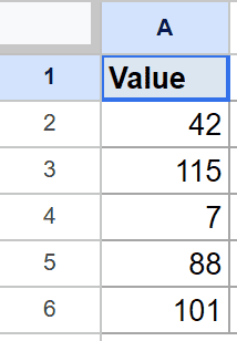
Example 3: Round Up to the Nearest Ten
A negative places argument rounds up to the left of the decimal point.
Below is the dataset. Column A holds a list of whole numbers we want rounded up to tidy tens.
I want each value rounded up to the nearest ten in column B.
Here is the formula:
=ROUNDUP(A2, -1)
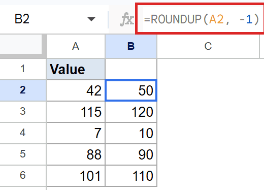
For 42, the formula returns 50. A places value of -1 rounds to tens, -2 would round to hundreds, and so on. Each value gets pushed up to the next ten, so 115 becomes 120 and 7 becomes 10.
This is great for rough planning numbers where you always want to round up to a clean figure rather than down.
Example 4: Round Up a Division to Whole Units
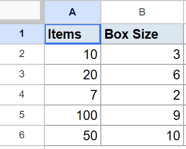
Here’s the example people reach for most. Working out how many containers you need.
Below is the dataset. Column A holds the number of items, and column B holds how many fit in one box.
I want to know how many boxes are needed for each row, with no item left behind.
Here is the formula:
=ROUNDUP(A2/B2, 0)
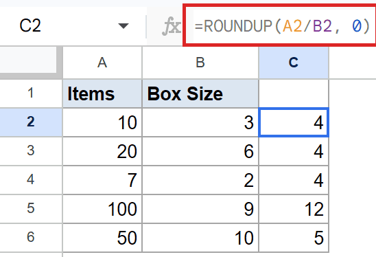
For 10 items in boxes of 3, the formula produces 4. Three boxes only hold 9, so you need a fourth box for the last item. Rounding down would leave that item homeless, which is why ROUNDUP is the right call here.
The division happens first, then ROUNDUP pushes the result up to the next whole box. This same pattern works for pages, batches, or any time a partial unit still needs a full one.
Pro Tip: If you want to round up to a multiple instead of a number of decimal places (say, up to the next 5 or 25), the CEILING function in Google Sheets does that in one step.
Tips & Common Mistakes
- ROUNDUP is not the same as ROUND. ROUND uses normal rounding, so 2.4 goes down to 2. ROUNDUP always goes up, so 2.4 goes to 3. Pick the one that matches what you actually need.
- Negative places round to the left. A places value of -1 rounds to tens and -2 to hundreds. It’s easy to forget the minus sign and end up rounding decimals instead.
- ROUNDUP rounds away from zero, both directions. With negative numbers, -2.1 rounds to -3, not -2. If you only want bigger-toward-positive behavior, reach for CEILING instead.
That’s the ROUNDUP function in Google Sheets. You’ve seen it round to whole numbers, to decimal places, up to the nearest ten, and up to whole boxes from a division.
Whenever rounding down would leave you short, ROUNDUP is the safe choice.
List of All Google Sheets Functions
Related Google Sheets Functions / Articles: