When you need to chop off decimals or round numbers toward zero without any “round half up” guesswork, the ROUNDDOWN function in Google Sheets does it predictably. This article walks through five examples covering whole numbers, decimals, negative places, and a discount calculation.
ROUNDDOWN Function Syntax in Google Sheets
The function takes a number and an optional places argument.
=ROUNDDOWN(value, [places])
- value – the number you want to round down toward zero
- places – the number of decimal places to keep; positive keeps decimals, zero gives a whole number, negative rounds to tens, hundreds, etc., [optional]
ROUNDDOWN always truncates toward zero, so 12.7 becomes 12 and -12.7 becomes -12.
When to Use ROUNDDOWN Function
- Trimming a decimal column to whole numbers without rounding up
- Cutting prices down to a fixed number of cents
- Rolling values down to the nearest ten, hundred, or thousand
- Calculating discounted totals that always round in the customer’s favor
- Cleaning up long decimals from other formulas for a tidier display
Example 1: Round decimals down to a whole number
Let’s start with the most common case, knocking the decimal part off a column of numbers.
Below is the dataset, with values 12.7, 4.3, 99.99, 0.5, and 25.01 in A2 to A6.
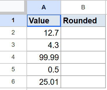
The goal is to drop the decimal in every cell and keep only the integer portion.
Here is the formula:
=ROUNDDOWN(A2, 0)
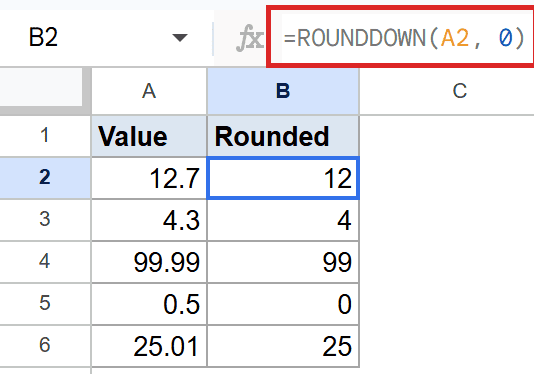
Setting places to 0 tells ROUNDDOWN to keep zero decimals. The result for A2 is 12. Drag the formula down and you’ll see 4, 99, 0, and 25.
Note that 0.5 rounds down to 0, not 1, because ROUNDDOWN ignores the standard “0.5 rounds up” rule.
Pro Tip: TRUNC behaves nearly identically to ROUNDDOWN with places=0. ROUNDUP is the opposite direction, ROUND is the standard half-up rule, and FLOOR rounds toward negative infinity (different from ROUNDDOWN for negatives).
Example 2: Round prices down to two decimal places
Set places to 2 when you want to keep cents but kill fractional cents.
Below is the dataset, prices in A2 to A6 with three decimal places, like 12.789 and 4.321.
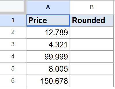
The goal is to trim each price to two decimals, always rounding down.
Here is the formula:
=ROUNDDOWN(A2, 2)
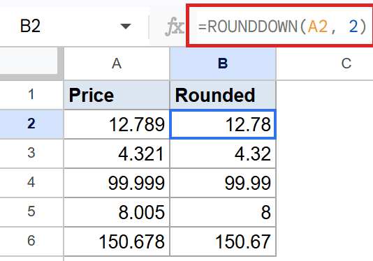
The result for A2 is 12.78. The third decimal is chopped off, not rounded. Drag the formula down and the rest of the column comes back as 4.32, 99.99, 8, and 150.67.
This is useful for invoice rounding when you want to be sure you never round a partial cent up.
Example 3: Round down to the nearest ten with negative places
The places argument also accepts negative numbers, which round to the left of the decimal point.
Below is the dataset, with values 47, 89, 123, 999, and 5 in A2 to A6.
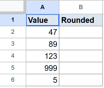
The goal is to round each number down to the nearest ten.
Here is the formula:
=ROUNDDOWN(A2, -1)
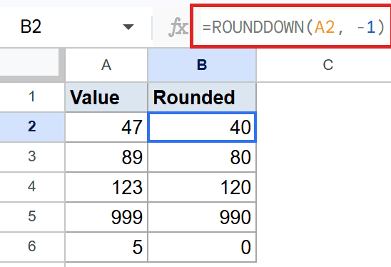
Setting places to -1 rounds to the tens place. The result for A2 is 40. The rest of the column comes back as 80, 120, 990, and 0 (because 5 rounded down to the nearest ten is 0).
Use -2 for the nearest hundred, -3 for the nearest thousand, and so on.
Example 4: Round negative numbers toward zero
ROUNDDOWN’s behavior on negatives is the main thing that separates it from FLOOR. ROUNDDOWN moves toward zero, while FLOOR moves further from zero.
Below is the dataset, negative values -12.7, -4.3, -0.9, -99.99, and -1.5 in A2 to A6.
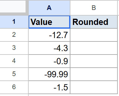
The goal is to trim each negative value to a whole number, always toward zero.
Here is the formula:
=ROUNDDOWN(A2, 0)
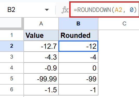
How this formula works:
- ROUNDDOWN truncates toward zero regardless of sign.
- -12.7 becomes -12, not -13.
- FLOOR(-12.7) would give -13 (further from zero), but ROUNDDOWN goes the other way.
The rest of the column comes back as -4, 0, -99, and -1.
Example 5: Apply a discount and round down to whole dollars
ROUNDDOWN works well wrapped around a calculation, like a discount that should always favor the customer.
Below is the dataset, original prices in column A from A2 to A6, mixing whole numbers and decimals like 49.99 and 12.50.
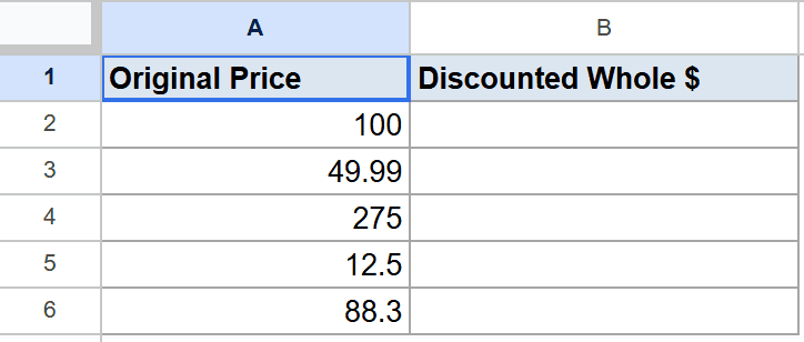
The goal is to apply a 15% discount and round each result down to whole dollars, so customers always pay less.
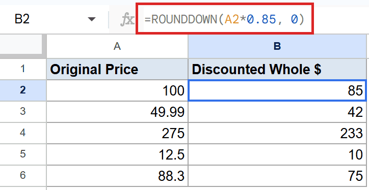
Here is the formula:
=ROUNDDOWN(A2*0.85, 0)
How this formula works:
- A2*0.85 applies the 15% discount (multiplying by 0.85 keeps 85% of the original).
- ROUNDDOWN with places 0 drops the decimal off the discounted result.
- For A2 (100), the math is 85, and the formula returns 85.
- The rest of the column comes back as 42, 233, 10, and 75.
The pattern works with SUM function too, like =ROUNDDOWN(SUM(A2:A6), 0) when you want a clean integer total.
Tips & Common Mistakes
- Watch the sign on the places argument. Positive numbers count decimal places, zero gives whole numbers, and negatives round to tens, hundreds, thousands.
- ROUNDDOWN is not FLOOR. For negatives, ROUNDDOWN goes toward zero and FLOOR goes further from it. Pick whichever direction matches your intent.
- Pair with IF function for conditional rounding. Wrap ROUNDDOWN inside IF when only some rows should be truncated and others left alone.
ROUNDDOWN is the predictable choice when you don’t want any half-up surprises. The places argument handles decimals, whole numbers, and tens-and-above with one syntax. Just remember the toward-zero behavior on negatives is the key difference from FLOOR.
List of All Google Sheets Functions
Related Google Sheets Functions / Articles: