
If you want one formula to work across a whole column instead of copying it down every row, the ARRAYFORMULA function in Google Sheets does that for you.
You write the calculation once, point it at a range, and the results spill down on their own. In this article I’ll show you how it works with five examples.
ARRAYFORMULA Function Syntax in Google Sheets
Here is how you write the ARRAYFORMULA function.
=ARRAYFORMULA(array_formula)
- array_formula – a single value, a range, or an expression made of ranges that returns a result the same size as its inputs. ARRAYFORMULA applies it to every row at once.
When to Use ARRAYFORMULA Function
- Run a calculation down a whole column without copying a formula into each cell.
- Multiply, add, or combine two columns row by row in one formula.
- Join text from several columns across every row at once.
- Keep results updating automatically as new rows of data come in.
Example 1: Multiply Two Columns at Once
Let’s start with the most common use, multiplying two columns together.
Below is the dataset, quantities in column A and prices in column B, rows 2 to 6.
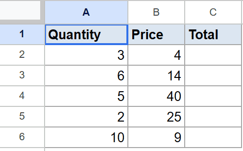
The goal is to get the total for each row without filling a formula down column C.
Here is the formula:
=ARRAYFORMULA(A2:A6*B2:B6)
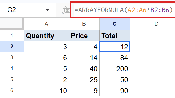
ARRAYFORMULA takes the two ranges, multiplies them row by row, and spills each result into column C. One formula in C2 fills all five rows.
The first row gives 12, the second 84, and the rest follow the same pattern. You never touch C3 through C6.
Example 2: Join First and Last Names
Here’s how to combine text from two columns in a single formula.
Below is the dataset, first names in column A and last names in column B, rows 2 to 5.
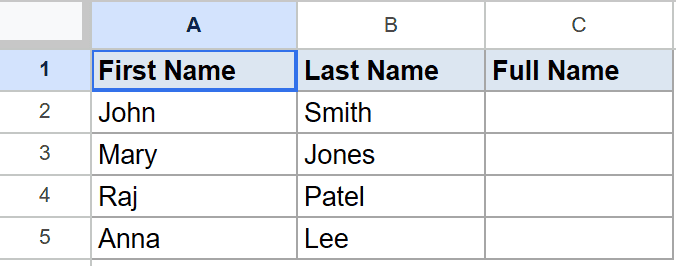
The goal is to build a full name for every row at once.
Here is the formula:
=ARRAYFORMULA(A2:A5&" "&B2:B5)
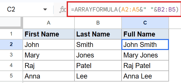
The & joins the two text values, and the " " drops a space between them. ARRAYFORMULA repeats that across every row.
So the first row reads John Smith and the second reads Mary Jones. The whole column fills from one formula.
Example 3: Apply an IF Test Across a Column
ARRAYFORMULA also lets you run a logical test down a whole column.
Below is the dataset, student names in column A and their scores in column B, rows 2 to 6.
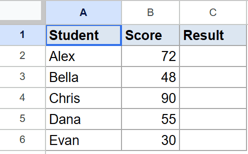
The goal is to mark each student Pass or Fail based on their score.
Here is the formula:
=ARRAYFORMULA(IF(B2:B6>=50,"Pass","Fail"))
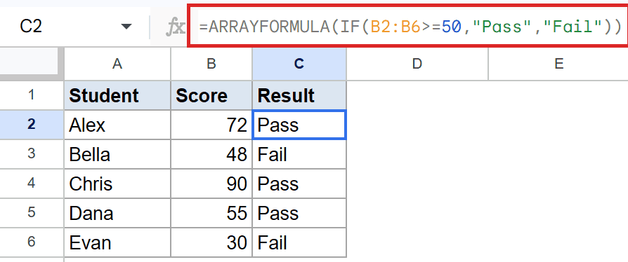
Normally IF checks one cell. Wrapping it in ARRAYFORMULA lets that same test run against every score in the range.
A score of 50 or more returns Pass, anything below returns Fail. The first student passes, the second fails, and so on down the column.
Pro Tip: ARRAYFORMULA is what makes IF work over a range. A plain IF only checks one cell, so without the wrapper you would have to copy it down row by row.
Example 4: Count Characters in Every Cell
You can wrap most text functions in ARRAYFORMULA too.
Below is the dataset, a single column of words in A2 to A6.
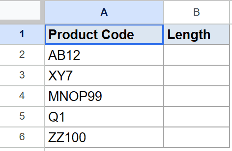
The goal is to count the characters in each word in one formula.
Here is the formula:
=ARRAYFORMULA(LEN(A2:A6))
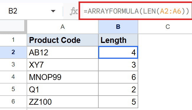
On its own the LEN function counts characters in a single cell. Wrap LEN in ARRAYFORMULA and it counts every cell in the range at once.
A four-letter word returns 4, a three-letter word returns 3, and the count drops into column B for every row.
Example 5: Calculate a Percentage for Each Row
Last one, scaling a column of numbers by a fixed factor.
Below is the dataset, item names in column A and sales values in column B, rows 2 to 5.
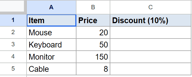
The goal is to work out a 10 percent commission on every sale at once.
Here is the formula:
=ARRAYFORMULA(B2:B5*0.1)
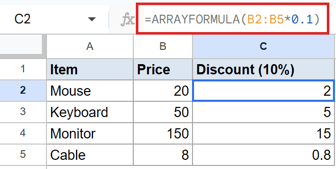
Multiplying the range by 0.1 takes ten percent of each sales value. ARRAYFORMULA runs that math down the whole column.
The first sale returns 2 and the second returns 5. Change a sales figure and its commission updates straight away.
Tips & Common Mistakes
- Your ranges need to be the same size. If column A runs to row 6 and column B only to row 5, the math falls out of line and you get the wrong answer.
- Leave the cells below your formula empty. ARRAYFORMULA spills into them, and any existing value blocks the spill with a #REF! error.
- You don’t always need to type it out. Select the cell, type your formula, and press Ctrl + Shift + Enter, and Google Sheets wraps it in ARRAYFORMULA for you.
ARRAYFORMULA is the function to reach for whenever you’d otherwise copy a formula down a column. You write the logic once and it handles every row.
It works with math, text joins, IF tests, and most other functions, and the results refresh on their own as your data grows.
List of All Google Sheets Functions
Related Google Sheets Functions / Articles: