
If you need to check whether a cell holds the #N/A error, the ISNA function in Google Sheets gives you a clean TRUE or FALSE. You point it at a cell or a formula, and it tells you if the result is that specific error.
In this article, I’ll show you how to use ISNA on plain cells, with MATCH, inside an IF wrapper, and directly on top of a VLOOKUP.
ISNA Function Syntax in Google Sheets
The ISNA function tests a value or formula and returns TRUE only when the result is the #N/A error.
=ISNA(value)
- value is the cell, value, or formula you want to test. ISNA returns TRUE only for #N/A, and FALSE for everything else, including other error types like #REF! or #VALUE!.
When to Use ISNA Function
- Flag lookup formulas that came back with no match instead of showing the raw error.
- Build cleaner conditional formatting that highlights only the #N/A cells.
- Replace error values with friendly text by combining ISNA with the IF function.
- Audit a column of formulas and count exactly how many failed with #N/A.
- Filter out missing-record rows before running totals or averages.
Example 1: Spot Cells That Hold the N/A Error
Let’s start with the simplest case, checking plain cells one at a time.
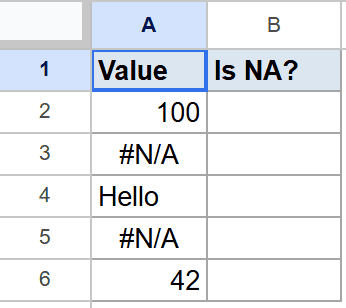
Below is the dataset. Column A has a mix of numbers, text, and two cells that contain =NA() which forces the #N/A error.
I want a TRUE or FALSE in column B that flags every #N/A cell.
Here is the formula:
=ISNA(A2)
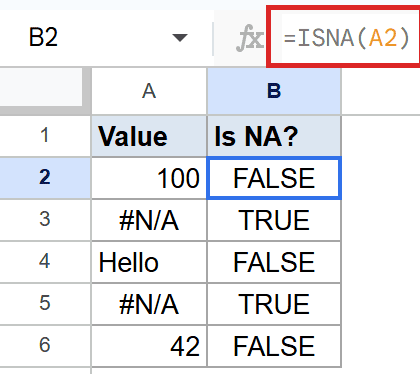
ISNA looks at each cell and returns TRUE only when the value is #N/A. The number, the text, and the other number all come back FALSE. The two =NA() cells return TRUE.
This is the cleanest way to scan a column for #N/A without writing any extra logic.
Example 2: Flag Names Missing From a Roster With MATCH
ISNA gets useful fast when paired with the MATCH function. MATCH returns #N/A when a value isn’t in the list, which is exactly what ISNA looks for.
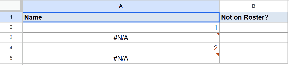
Below is the dataset. Column A has four MATCH formulas, each checking whether a name appears in a small roster of Alice, Bob, and Carol.
I want column B to say TRUE for any name that isn’t on the roster.
Here is the formula:
=ISNA(A2)
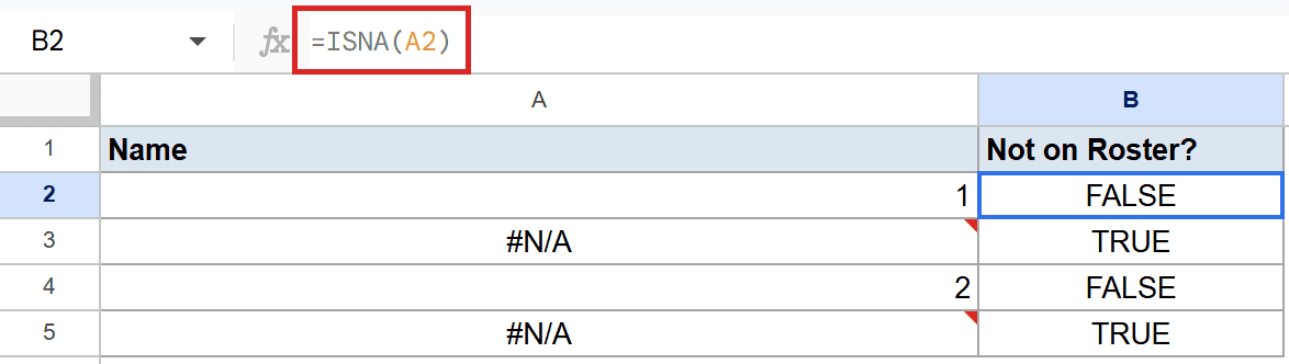
Alice and Bob are on the roster, so their MATCH calls return a position number and ISNA reports FALSE. Dave and Eve aren’t on the roster, so MATCH gives #N/A and ISNA flips it to TRUE.
This pattern is the easiest way to do a membership check on a list. ISNA turns the error into a clean boolean you can use in further logic.
Example 3: Replace N/A With a Friendly Message
Wrap ISNA inside an IF and you can swap the error for any readable label.
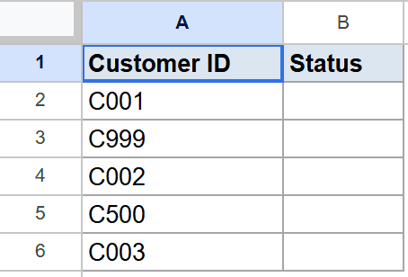
Below is the dataset. Column A has five customer IDs, and the formula in column B looks each one up in a mini-table of C001 through C003.
I want the lookup result if there’s a match, or the text “Not Found” if there isn’t.
Here is the formula:
=IF(ISNA(VLOOKUP(A2, {"C001","Alice";"C002","Bob";"C003","Carol"}, 2, FALSE)), "Not Found", VLOOKUP(A2, {"C001","Alice";"C002","Bob";"C003","Carol"}, 2, FALSE))

Here’s how this formula works:
- The inner VLOOKUP tries to find the customer ID in the mini-table.
- ISNA checks whether that lookup came back with #N/A.
- If yes, IF returns the text “Not Found”. If no, IF runs the VLOOKUP again and returns the matched name.
C001, C002, and C003 all match, so you see Alice, Bob, and Carol. C999 and C500 aren’t in the table, so both rows show Not Found instead of the raw error.
Pro Tip: If you only need a fallback for #N/A and don’t care about inspecting the error type, IFNA does the same job in one call. Use IFERROR if you want to catch every kind of error, not just #N/A.
Example 4: Wrap a VLOOKUP Directly to Check for Misses
You don’t need an extra column of lookup results. ISNA can sit right on top of the lookup.
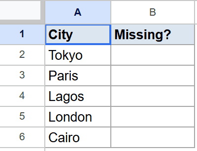
Below is the dataset. Column A has five city names, and the formula in column B looks each city up in a region table of Tokyo, London, and Sydney.
I want TRUE in column B for every city that isn’t in the lookup table.
Here is the formula:
=ISNA(VLOOKUP(A2, {"Tokyo","Asia";"London","Europe";"Sydney","Oceania"}, 2, FALSE))
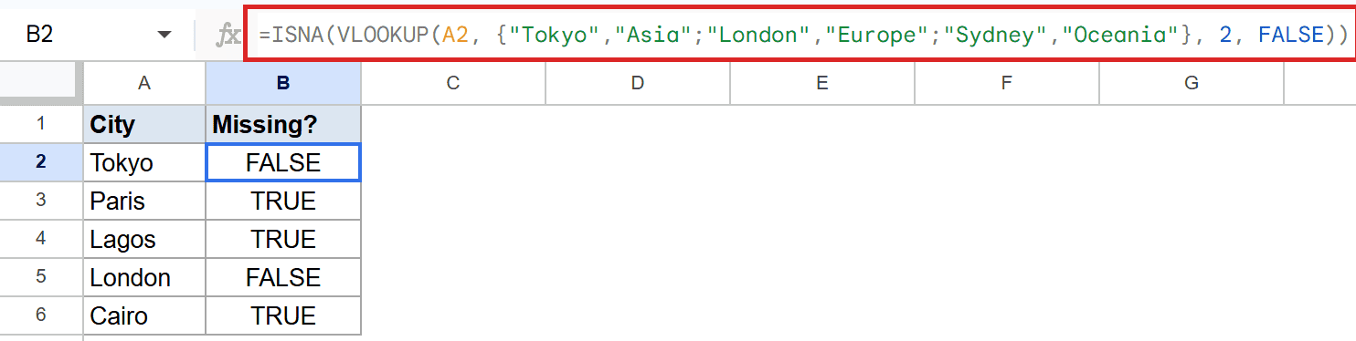
Tokyo and London are in the table, so VLOOKUP succeeds and ISNA returns FALSE. Paris, Lagos, and Cairo aren’t there, so the VLOOKUP fails with #N/A and ISNA reports TRUE.
This is great for audits. You can quickly highlight which rows in a list don’t exist in your reference data without a helper column.
Tips & Common Mistakes
- ISNA only catches #N/A, nothing else. Errors like #REF!, #VALUE!, or #DIV/0! all come back as FALSE from ISNA. If you want to catch any kind of error, use ISERROR or IFERROR instead.
- You can pass a formula directly, not just a cell reference.
=ISNA(VLOOKUP(...))is a common shortcut that skips the helper column entirely. - For shorter formulas, IFNA is a one-call alternative. Where
=IF(ISNA(X), "Not Found", X)repeats X twice,=IFNA(X, "Not Found")writes it once. Use ISNA when you want a clean TRUE/FALSE result rather than a substituted value.
ISNA is a small function, but it makes the #N/A error a lot easier to work around.
You’ve now seen it tested against plain cells, used with MATCH, wrapped inside IF for friendly messages, and dropped on top of VLOOKUP. Pick the shape that fits your sheet.
List of All Google Sheets Functions
Related Google Sheets Functions / Articles: