
CHOOSE returns an option based on its position in a list. An index of 1 selects the first option, 2 selects the second, and so on. Use it for short lists of sequential numeric codes.
CHOOSE function syntax
=CHOOSE(index, choice1, [choice2, ...])- index: the position to select, starting at 1. Use a whole number within the supplied choices.
- choice1 and additional choices: text, numbers, cell references or expressions to select. Text labels need quotation marks.
- In our Google Sheets test, the highest usable index was 29. Index 30 returned #NUM! even with 30 choices supplied.
Set up the example data
Enter this dataset starting in A1. The first row contains headings. Keep the result area separate from the source table.
| Code | Sales |
|---|---|
| 1 | 10000 |
| 3 | 25000 |
| 2 | 15000 |
| 4 | 20000 |
Turn status codes into labels
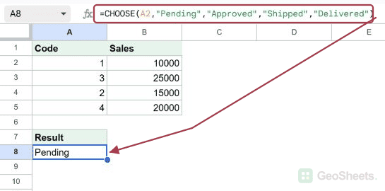
Enter this formula in A8. Code 1 in A2 selects Pending. For a list beside the input, enter the same formula in C2 and fill down through C5.
=CHOOSE(A2,"Pending","Approved","Shipped","Delivered")Result: Pending.
Return all status labels with one formula
Enter this version in an empty output area. It returns four labels in input order: Pending, Shipped, Approved and Delivered. The A1 header is deliberately excluded.
=ARRAYFORMULA(CHOOSE(A2:A5,"Pending","Approved","Shipped","Delivered"))Result: Pending; Shipped; Approved; Delivered.
Select a calculation using a mode number
Here the mode is 3. The choices are addition, subtraction, multiplication and division, so this example selects 10 multiplied by 5. Replace 3 with a cell reference for an editable mode.
=CHOOSE(3,10+5,10-5,10*5,10/5)Result: 50.
Calculate commission from a tier number
Treat the codes in column A as commission tiers for this example. Tier 1 uses 5%, tier 2 uses 8%, tier 3 uses 10%, and tier 4 uses 15%. Multiply the selected rate by sales.
=B2*CHOOSE(A2,0.05,0.08,0.1,0.15)Result: 500.
Convert a weekday number into a custom name
WEEKDAY uses Sunday = 1 by default. January 1, 2026 is Thursday, which selects the fifth label. DATE creates an actual date without depending on how typed date text is interpreted.
=CHOOSE(WEEKDAY(DATE(2026,1,1)),"Sun","Mon","Tue","Wed","Thu","Fri","Sat")Result: Thu.
Choose which quarter to sum
Enter the regional sales table at A20. The index 3 selects D21:D24, the Q3 column. SUM then adds 150, 220, 200 and 190. Replace 3 with a quarter-input cell when needed.
| Region | Q1 | Q2 | Q3 | Q4 |
|---|---|---|---|---|
| East | 100 | 120 | 150 | 170 |
| West | 180 | 200 | 220 | 240 |
| North | 160 | 180 | 200 | 220 |
| South | 150 | 170 | 190 | 210 |
=SUM(CHOOSE(3,B21:B24,C21:C24,D21:D24,E21:E24))Result: 760.
Other Google Sheets articles you may also like