INDIRECT Function in Google Sheets

If you have a cell reference written as plain text and you want Google Sheets to treat it as a real reference, the INDIRECT function is what you need. It turns a text string like "B2" into a live link to that cell and pulls the value sitting there.

In this article, I’ll walk you through five practical examples, including a plain text address, building a reference from a row number, summing a named range, R1C1 notation, and switching columns on the fly.

INDIRECT Function Syntax in Google Sheets

INDIRECT takes a text reference and an optional flag for which notation that text uses.

=INDIRECT(reference_as_string, [is_A1_notation])

• reference_as_string: the cell or range reference written as text, like "B2" or "A1:A10". Can be a literal string or built from other cells.
• is_A1_notation (optional): TRUE (the default) reads the text as A1 notation. FALSE reads it as R1C1 notation.

When to Use INDIRECT Function

• Convert a text address typed in a cell into the actual value at that cell.
• Build a reference dynamically by joining text with a row or column number.
• Point SUM, AVERAGE, or COUNT at a range whose name lives in another cell.
• Switch which column a formula reads based on a dropdown or input cell.
• Reference a named range by passing its name as text.

Example 1: Resolve a plain text address

Let’s start with the simplest case. You have cell addresses typed as text and you want the value each one points to.

Below is the dataset with fruit names in column A, text addresses in column B, and an empty result column C.

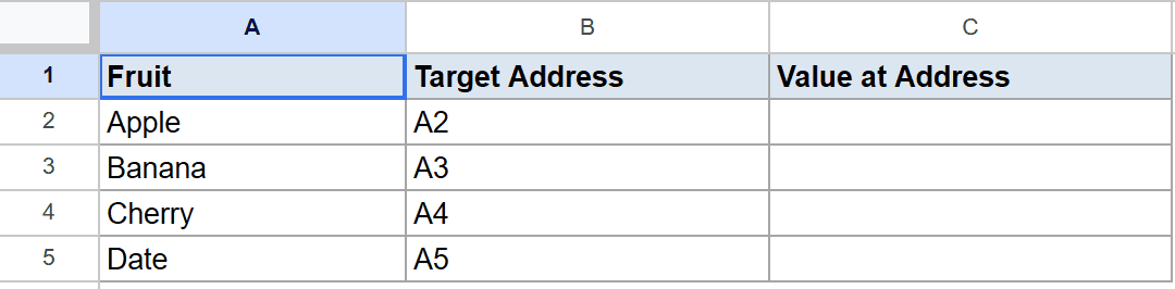
The goal is to read the address in column B and return whatever value lives at that cell.

Here is the formula:

=INDIRECT(B2)

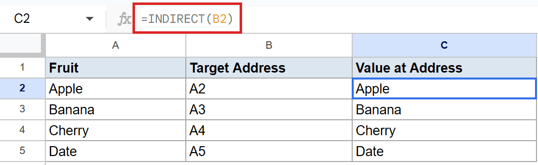
B2 holds the text A2, so INDIRECT points at cell A2 and returns Apple. Filling down, B3 points at A3 to return Banana, then Cherry and Date follow.

The text in column B is just a string. INDIRECT is what makes Google Sheets treat it as a real reference instead of plain text.

Example 2: Build a reference from a row number

Often you don’t have the full address, just a row number. You can join a column letter with that number to build the reference.

Below is the dataset with row numbers in column A and product names in column B, with column C empty.

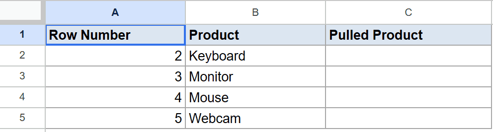
The goal is to pull the product name from column B using the row number sitting in column A.

Here is the formula:

=INDIRECT("B"&A2)

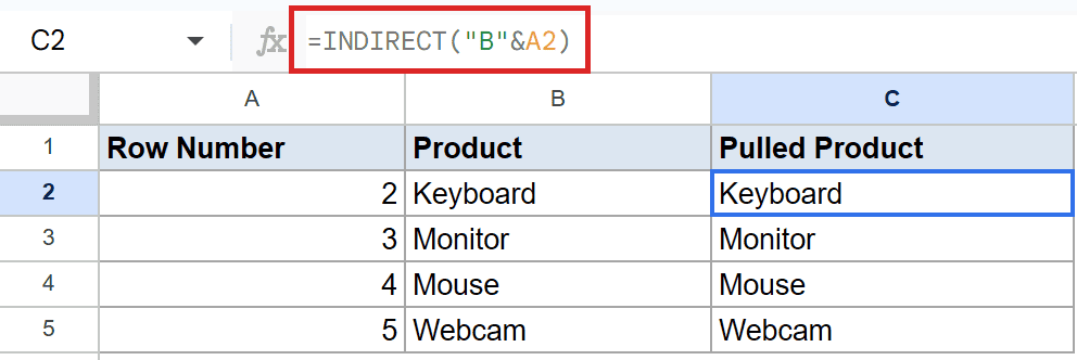
How this formula works:

• "B"&A2 joins the letter B with the number in A2. If A2 holds 2, the text becomes B2.
• INDIRECT turns that text into a live reference and returns the value at B2, which is Keyboard.
• Filling down builds B3, B4, and B5, returning Monitor, Mouse, and Webcam.

Pro Tip: Joining a column letter with a number is the most common INDIRECT pattern. Swap the letter for another cell to make both the column and the row dynamic.

Example 3: Sum a named range passed as text

INDIRECT can also resolve a named range. This is handy when the name you want to total is stored as text in a cell.

Below is the dataset where column A holds a named range called Sales and column B holds the values inside it, with the range name typed in A2.

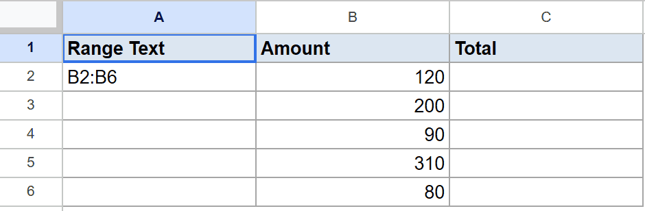
The goal is to total the named range whose name is sitting in cell A2.

Here is the formula:

=SUM(INDIRECT(A2))

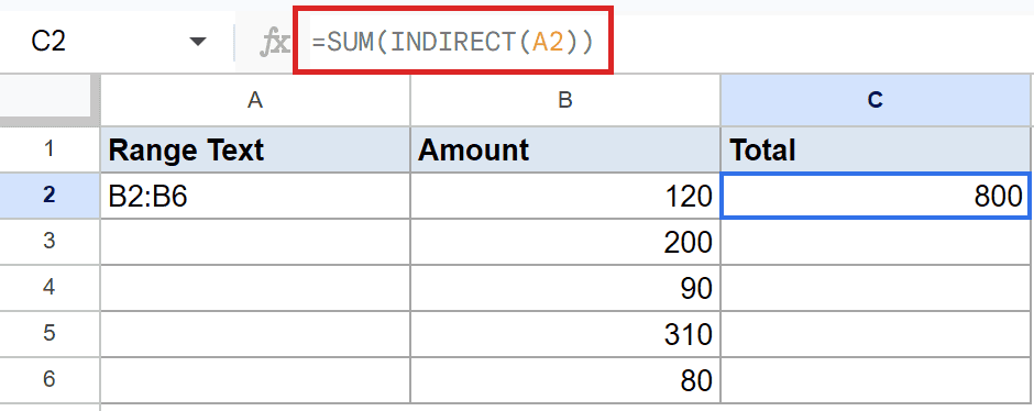
A2 holds the text Sales, which is the name of a defined range. INDIRECT resolves that text into the actual range, and SUM adds up its values to return 800.

This works because INDIRECT accepts named ranges just like it accepts cell addresses. The name simply needs to exist in the sheet. You can use the same idea with the ADDRESS function when you want to build the address text first and resolve it second.

Example 4: Reference a cell using R1C1 notation

INDIRECT can read addresses written in R1C1 notation, where you give a row number and a column number instead of a letter and a number.

Below is the dataset with a small grid of values in columns A through C, plus a result cell in column D.

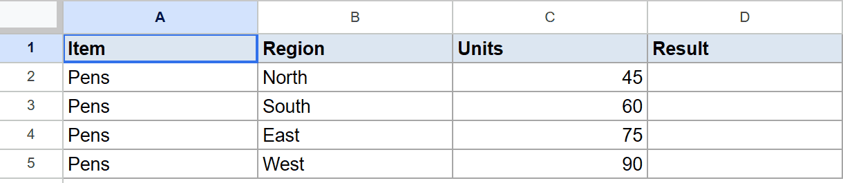
The goal is to grab the value at row 5, column 3 using R1C1 notation.

Here is the formula:

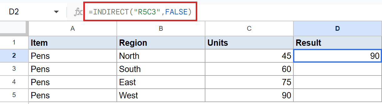
=INDIRECT("R5C3",FALSE)

How this formula works:

• "R5C3" means row 5, column 3, which is cell C5 in normal A1 notation.
• The second argument FALSE tells INDIRECT to read the text as R1C1 instead of A1.
• The value at C5 is 90, so that’s what comes back.

Pro Tip: R1C1 is useful when you already have row and column numbers from functions like the [ROW](https://geosheets.com/google-sheets-function/row/) and COLUMN functions, since you can build the address as numbers without converting to letters first.

Example 5: Switch columns on the fly

This is the example that shows INDIRECT at its most flexible. You can let an input cell decide which column a formula totals.

Below is the dataset with monthly figures across columns B through D and an input cell in B5 that names a column letter.

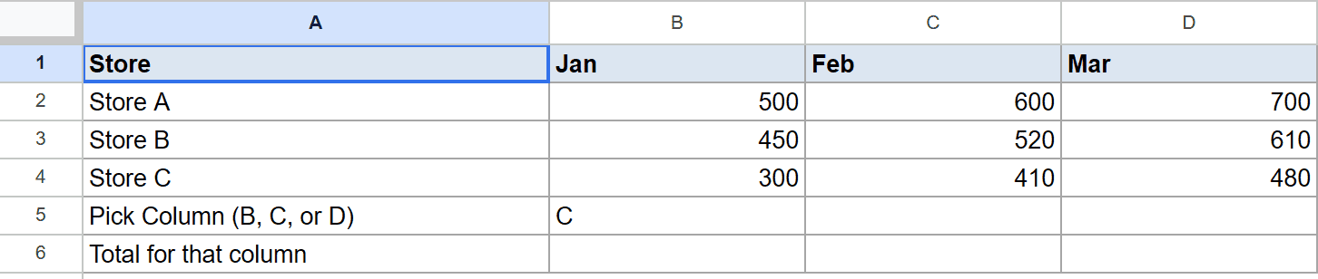
The goal is to total rows 2 through 4 of whichever column letter is typed into B5.

Here is the formula:

=SUM(INDIRECT(B5&"2:"&B5&"4"))

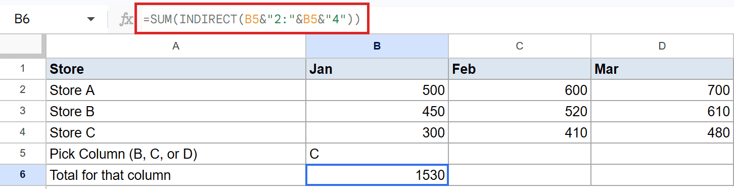
How this formula works:

• B5 holds a column letter. The formula joins it into a range like C2:C4.
• INDIRECT turns that text into a real range, and SUM totals the three values.
• With the current input the total is 1530. Change the letter in B5 and SUM re-points at a different column.

This is a clean way to build a column switcher without rewriting the formula each time.

Tips & Common Mistakes

• INDIRECT is volatile. It recalculates on almost every change to the sheet, even edits unrelated to it. On large sheets with many INDIRECT formulas this can slow things down noticeably.
• INDIRECT does not follow cells when you move them. Because it points at a literal text address, moving the referenced cell leaves INDIRECT pinned to the original location. That is usually the whole point, but it surprises people who expect a normal reference.
• Watch your quotes and notation. A reference like B2 must be passed as text, either as "B2" or built from cells. If you pass R1C1 text, remember to set the second argument to FALSE.

INDIRECT looks small, but it bridges the gap between text and real references. Once you can build an address as text and hand it back as a live reference, dynamic column switchers and name-driven sums become easy. It pairs naturally with the ADDRESS function and the COLUMN function when you need to assemble references from parts.

List of All Google Sheets Functions

Related Google Sheets Functions / Articles:

• INDEX Function in Google Sheets
• OFFSET Function in Google Sheets
• ROW Function in Google Sheets
• CHOOSE Function in Google Sheets
• COLUMNS Function in Google Sheets