
If you want to find a value in one list and pull back the matching value from another list, the LOOKUP function in Google Sheets does it in a single, simple call.
The one rule to remember is that LOOKUP needs your search range sorted in ascending order. In this article, I’ll walk you through five examples covering numeric lookups, text results, the array form, and a horizontal lookup across rows.
LOOKUP Function Syntax in Google Sheets
LOOKUP comes in two shapes. The first searches one range and returns from a parallel range.
=LOOKUP(search_key, search_range, [result_range])
search_key: the value you’re looking for.search_range: the range to search through. This must be sorted in ascending order.result_range(optional): the range to pull the matching value from. It should be the same size as the search range.
If you leave out result_range, LOOKUP switches to its array form. It searches the first column (or row) of the range and returns the value from the last column (or row) of the matched position.
One thing worth knowing up front. LOOKUP does not look for an exact match. It returns the largest value that is less than or equal to your search key, which is why the search range has to be sorted.
When to Use LOOKUP Function
- Match a value against a sorted list and pull a result from a parallel column.
- Assign a bracket or band, such as a grade or shipping tier, based on a sorted threshold table.
- Pull the matching value when your lookup column sits to the right of the result column.
- Search a single horizontal row and return from the row beneath it.
- Build a quick lookup without worrying about column index numbers.
Example 1: Look up a price from a sorted quantity table
Let’s start with the most common case, a numeric lookup against a sorted table.
Below is the dataset with quantity breakpoints in column A, their unit prices in column B, and the quantities you want to price in column C.
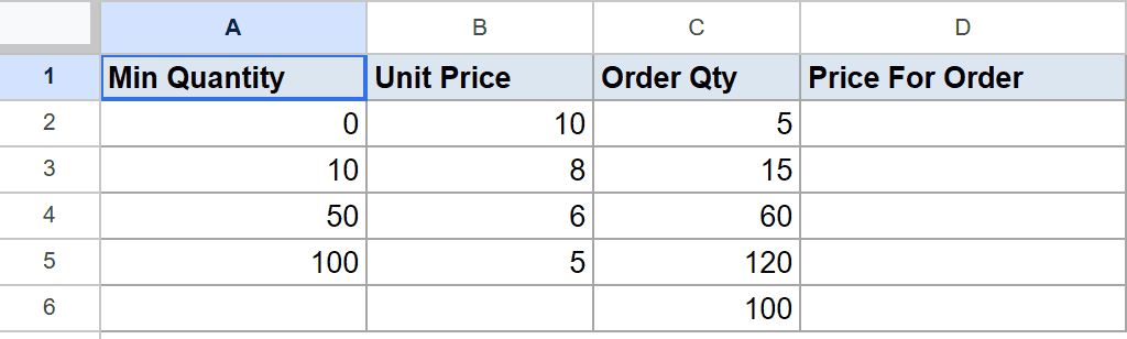
The goal is to return the matching unit price for each quantity in column C.
Here is the formula:
=LOOKUP(C2,$A$2:$A$5,$B$2:$B$5)
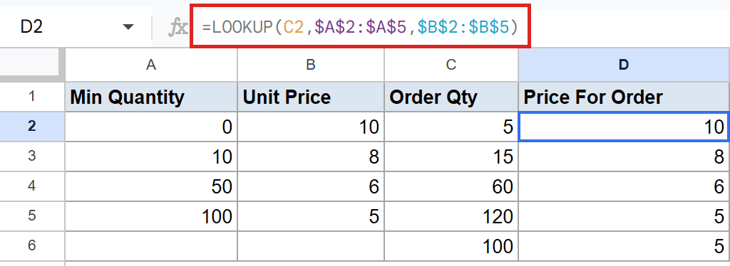
How this formula works:
- LOOKUP takes the quantity in C2 and scans the sorted breakpoints in column A.
- It finds the largest breakpoint that is less than or equal to that quantity.
- It then returns the price sitting in the same row of column B.
The five quantities return 10, 8, 6, 5, and 5. When a quantity falls between two breakpoints, LOOKUP rounds down to the lower breakpoint and grabs that price.
Pro Tip: LOOKUP only works correctly when the search range is sorted ascending. If your data isn’t sorted, sort it first or switch to the [HLOOKUP](https://geosheets.com/google-sheets-function/hlookup/) function for horizontal lookups, where you can force an exact match.
Example 2: Return a text result instead of a number
LOOKUP doesn’t care whether the result is a number or text. Here we return a letter grade.
Below is the dataset with score thresholds in column A, the matching grade letters in column B, and the scores to grade in column C.
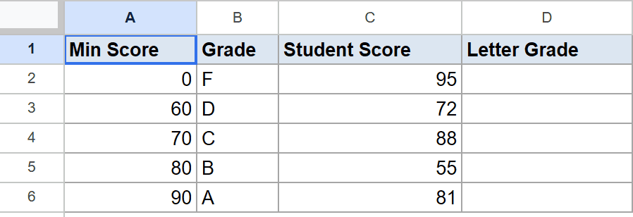
The goal is to assign a grade to each score in column C.
Here is the formula:
=LOOKUP(C2,$A$2:$A$6,$B$2:$B$6)
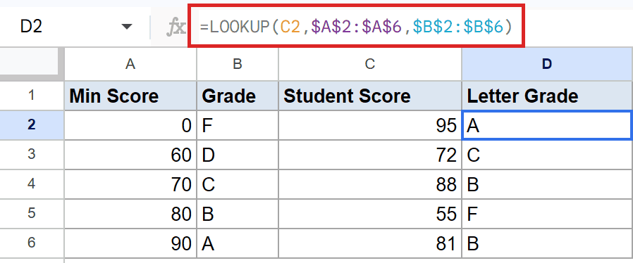
LOOKUP scans the sorted thresholds in column A and finds the highest one each score reaches. It then returns the grade from column B for that row.
The five scores come back as A, C, B, F, and B. A score that lands between two thresholds takes the grade of the lower threshold it clears.
Example 3: Use the array form to return the last column
When you skip the result range, LOOKUP reads a whole block and returns from its last column. This is the array form.
Below is the dataset with employee IDs in column A, their department names in column B, and the IDs to look up in column C.
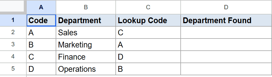
The goal is to return each looked-up ID’s department using a single range instead of two.
Here is the formula:
=LOOKUP(C2,$A$2:$B$5)
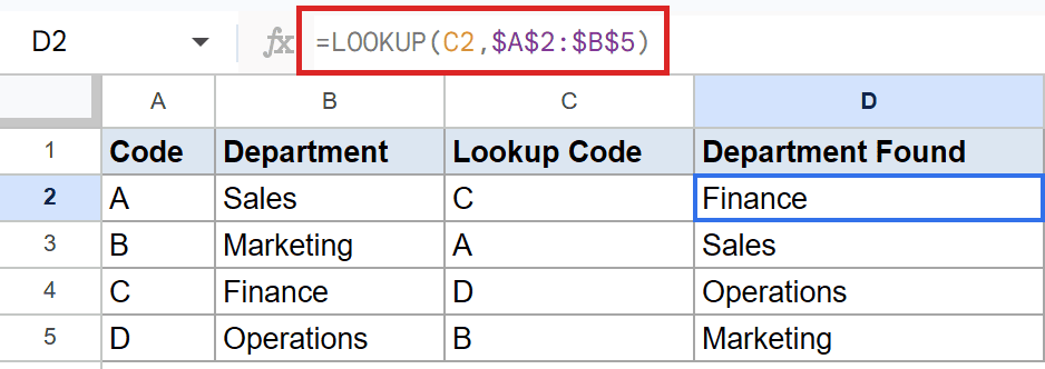
How this formula works:
- With only one range passed, LOOKUP searches the first column of
A2:B5, which holds the IDs. - It finds the matching row using the same largest-value-less-than-or-equal rule.
- It then returns the value from the last column of the range, which is the department in column B.
The four IDs return Finance, Sales, Operations, and Marketing. The array form is handy when your result column is simply the rightmost one in the block.
Pro Tip: The array form always returns from the last column of the range, so it only fits when your result sits on the far right. For anything more flexible, VLOOKUP or XLOOKUP lets you point at any column by index or by name.
Example 4: Assign a shipping band from a threshold table
This is the classic banding pattern. You sort your cutoffs ascending and let LOOKUP drop each value into the right band.
Below is the dataset with weight cutoffs in column A, the shipping fee for each band in column B, and the package weights in column C.
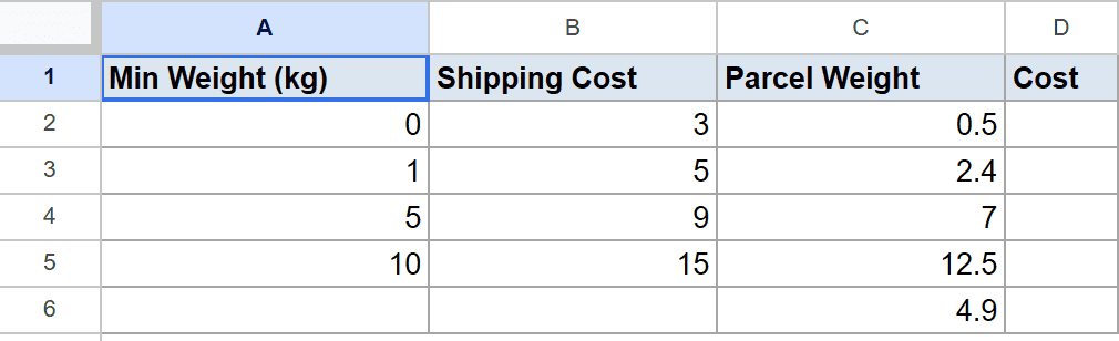
The goal is to find the shipping fee for each weight in column C.
Here is the formula:
=LOOKUP(C2,$A$2:$A$5,$B$2:$B$5)
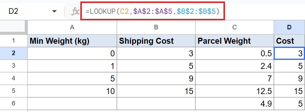
LOOKUP matches each weight to the highest cutoff it reaches and returns the fee from that row. The five weights return fees of 3, 5, 9, 15, and 5.
Notice how a weight sitting between two cutoffs takes the fee of the lower band. That is the ascending-sort rule doing its job.
Example 5: Look up across a horizontal row
LOOKUP can search a row instead of a column. Here the lookup keys run left to right across row 1.
Below is the dataset with quarter labels across row 1, their sales totals across row 2, and the quarter you want to find typed into B3.
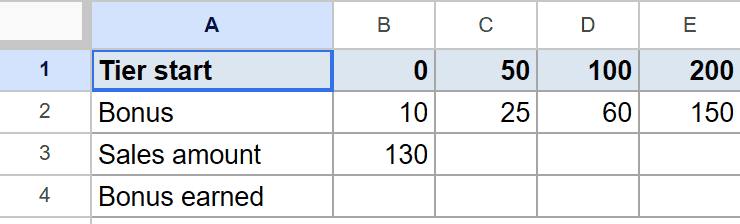
The goal is to pull the sales total for the quarter named in B3.
Here is the formula:
=LOOKUP(B3,B1:E1,B2:E2)
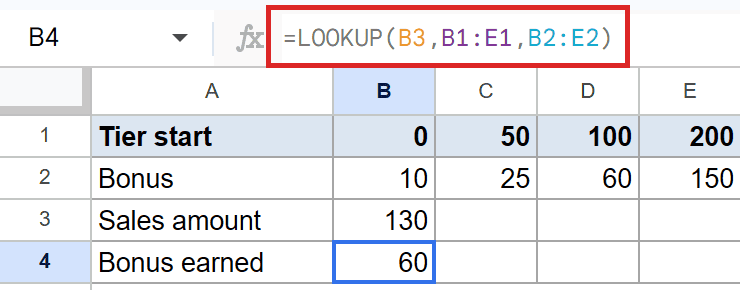
LOOKUP searches the quarter labels in B1:E1 and returns the matching total from the parallel row B2:E2. With Q3 in B3, the formula returns 60.
This horizontal form is the same idea as the column version, just rotated. The search row and the result row need to line up cell for cell.
Pro Tip: For a dedicated row-based lookup, the HLOOKUP function is usually clearer and lets you ask for an exact match. Reach for LOOKUP’s horizontal form only when your row is already sorted ascending.
Tips & Common Mistakes
- Sort the search range ascending. This is the number one cause of wrong LOOKUP results. On unsorted data, LOOKUP can return a value from the wrong row without throwing an error, so the mistake is easy to miss.
- LOOKUP is approximate by design. It never does an exact match. It returns the largest value less than or equal to your key, so if you need a strict exact match, use VLOOKUP, XLOOKUP, or the HLOOKUP function instead.
- Keep the search and result ranges the same size. If they don’t line up, the matched position won’t map to the right result. In the array form, remember the result always comes from the last column or row of the block.
LOOKUP is a quick way to match a value and pull back a result, whether your data runs down a column or across a row. Just keep the search range sorted and remember it returns the closest match at or below your key. For anything that needs an exact match or a flexible result column, the more robust lookup functions are the better pick.
List of All Google Sheets Functions
Related Google Sheets Functions / Articles: