XLOOKUP Function in Google Sheets

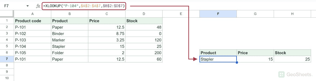
If you want to look up a value and pull back a match, but you’ve been fighting with VLOOKUP’s quirks, the XLOOKUP function is the cleaner option. You give it the value to find, the column to search, and the column to return from.

In this article, I’ll show you how XLOOKUP works in Google Sheets, with five examples covering left lookups, custom messages for missing values, approximate matching, and returning a whole row at once.

XLOOKUP Function Syntax in Google Sheets

Here is how the function is structured.

=XLOOKUP(search_key, lookup_range, result_range, [missing_value], [match_mode], [search_mode])
  • search_key – the value you want to find.
  • lookup_range – the single column or row that XLOOKUP searches through.
  • result_range – the column or row the result comes from. It lines up with the lookup range.
  • missing_value – what to show when nothing matches. Optional.
  • match_mode0 for exact (the default), -1 for next smaller, 1 for next larger. Optional.
  • search_mode – direction of the search. Optional, and rarely needed.

When to Use XLOOKUP Function

  • Pulling a value from a table without counting column positions like VLOOKUP needs.
  • Looking up a value that sits to the left of the result column.
  • Returning a clean message instead of an error when a lookup fails.
  • Finding the closest match below a threshold, like a tax bracket or shipping tier.
  • Returning a whole row of details from one lookup, which spills across several cells.

Example 1: Basic Lookup by Employee ID

Let’s start with the everyday case, matching an ID to a value.

Below is the dataset. Column A has employee IDs and column B has their department. Column D has a few IDs we want to look up.

Google Sheet showing Employee and Department data, plus Lookup Names, and an empty Department column.

We want to pull each employee’s department into column E.

Here is the formula:

=XLOOKUP(D2,$A$2:$A$6,$B$2:$B$6)
Google Sheets displaying an XLOOKUP formula in E2's formula bar, returning department data.

XLOOKUP takes the ID in D2, finds it in the lookup range $A$2:$A$6, then returns the matching value from the result range $B$2:$B$6. The first result comes back as Marketing.

Notice there’s no column number to count. You point at the lookup column and the result column directly, which is the big difference from VLOOKUP.

Pro Tip: XLOOKUP does an exact match by default, so you don’t have to remember a FALSE argument the way you do with VLOOKUP.

Example 2: Look to the Left

This is something VLOOKUP simply can’t do. With XLOOKUP, the result column can sit to the left of the lookup column.

Below is the dataset. Column A has product codes and column B has product names. Column D has the names we want to look up, and we want the code back.

Google Sheet: SKU/Item data in columns A-B, with Lookup Item values in column D.

We want to find each product name and return its code from the column to the left.

Here is the formula:

=XLOOKUP(D2,$B$2:$B$5,$A$2:$A$5)
Google Sheets showing XLOOKUP formula in E2: `=XLOOKUP(D2, $B$2:$B$5, $A$2:$A$5)`.

The lookup range is column B and the result range is column A. XLOOKUP doesn’t care which one is further left, so the search runs on the names and the codes come back. The first result is A-901.

With VLOOKUP you’d have to rearrange your columns or nest INDEX and MATCH to do this. XLOOKUP just handles it.

Example 3: Custom Message for No Match

When a lookup fails, XLOOKUP returns #N/A by default. But it has a built-in argument to show your own text instead, so you don’t need IFERROR.

Below is the dataset. Column A has country names and column B has their capitals. Column D has countries to look up, including a couple that aren’t in the list.

Google Sheet with Country and Capital columns, and a "Lookup Country" column.

We want the capital where the country exists, and a message where it doesn’t.

Here is the formula:

=XLOOKUP(D2,$A$2:$A$5,$B$2:$B$5,"No match")
XLOOKUP in Sheets E2 returns 'No match' for D2, using a custom missing value message.

The fourth argument is the missing value. When the country is found, you get the capital like Paris. When it isn’t, you get “No match” instead of an error.

This is one of XLOOKUP’s nicest touches. The fallback is built into the function, so there’s no extra wrapper to add.

Pro Tip: The missing_value argument only catches a no-match. It won’t hide other errors in the formula, so don’t treat it as a full replacement for IFERROR in every case.

Example 4: Approximate Match for Tiers

Sometimes you want the closest match below your lookup value, like fitting an order amount into a discount tier. The match_mode argument handles this.

Below is the dataset. Column A has order thresholds in ascending order, column B has the discount rate for each tier, and column D has order amounts to match.

Google Sheet showing Min Sales and Rate data, alongside Sales values for lookup.

We want the discount rate for each amount, using the next threshold at or below it.

Here is the formula:

=XLOOKUP(D2,$A$2:$A$5,$B$2:$B$5,,-1)
Google Sheets: XLOOKUP formula in E2 calculates rate for sales with approximate match (-1).

The -1 in the matchmode slot tells XLOOKUP to return the next smaller match when there’s no exact hit. The empty argument before it is the skipped missingvalue. The first amount returns a rate of 0.04.

Note the two commas before -1. That empty spot is the missingvalue argument we’re leaving blank so we can reach matchmode.

Example 5: Return a Whole Row at Once

Here’s where XLOOKUP really pulls ahead. The result range can be more than one column, so a single lookup returns an entire row of details.

Below is the dataset. Columns A through D hold an ID, age, city, and role. Cell F2 has the ID we want to look up.

Google Sheet with Name, Age, City, Title data; Riley in F2 for lookup, results empty.

We want every detail for that one ID, returned across cells in one go.

Here is the formula:

=XLOOKUP(F2,$A$2:$A$4,$B$2:$D$4)
Google Sheets: XLOOKUP formula in G2 returns spilled row '41 Denver Manager'.

The result range here is three columns wide, $B$2:$D$4. XLOOKUP finds the ID and returns the whole matching row, which spills into the cells to the right of the formula.

The result fills three cells: 41, Denver, and Manager. You write one formula and get the full record, instead of three separate lookups.

Pro Tip: For a row laid out sideways with the lookup keys in the top row, the HLOOKUP function is the horizontal lookup tool. XLOOKUP can also search a row, but HLOOKUP is the classic choice.

Tips & Common Mistakes

  • Lookup range and result range must be the same size. XLOOKUP lines them up row by row. If your lookup range is 5 cells tall and your result range is 4, you’ll get an error. Double-check the ranges match before filling down.
  • Don’t skip the missingvalue when you need matchmode. To use approximate match you have to leave the fourth argument empty with a comma, as in ...,$B$2:$B$5,,-1). Forgetting that empty slot shifts your arguments and breaks the result.
  • A single formula can return many cells. When the result range is more than one column wide, the answer spills. Make sure the cells to the right are empty, or you’ll get a spill block. The CHOOSE function is handy when you want to reorder which columns come back.

XLOOKUP cleans up most of the friction VLOOKUP carries, from looking to the left to building in a no-match message and returning a full row in one shot.

Once you’re used to pointing at the lookup column and result column directly, going back to counting column numbers feels like a step backward.

List of All Google Sheets Functions

Related Google Sheets Functions / Articles: