Apply Conditional Formatting Across Sheets in Google Sheets

You may keep your task list on one tab and its approval status on another. Or you might want sales figures to change color when they pass a target stored elsewhere in your spreadsheet.

In this tutorial, I’ll show you how to make those connections with conditional formatting. We’ll start with matching rows, then compare against a target and look up records that appear in a different order.

For another tab in the same spreadsheet, we’ll use INDIRECT inside the formatting rule. I’ll also explain the extra step you need when your source is a separate spreadsheet file.

Highlight rows using values on another tab

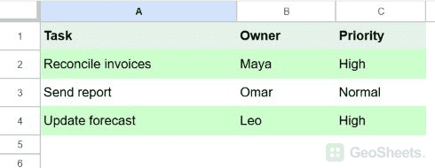
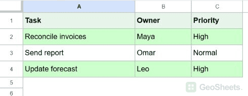
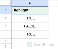
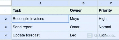
Below, I have three tasks on a tab named Sheet1. A second tab, Sheet2, contains a TRUE or FALSE value for each task. I want TRUE to highlight the corresponding task row.

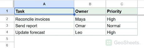
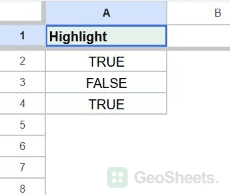
Enter TRUE and FALSE without quotation marks. Default checkboxes can supply these values too: a checked box is TRUE and an unchecked box is FALSE.

Let’s create the formatting rule on the task tab.

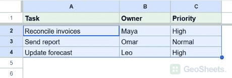
1. On Sheet1, select A2:C4.

   

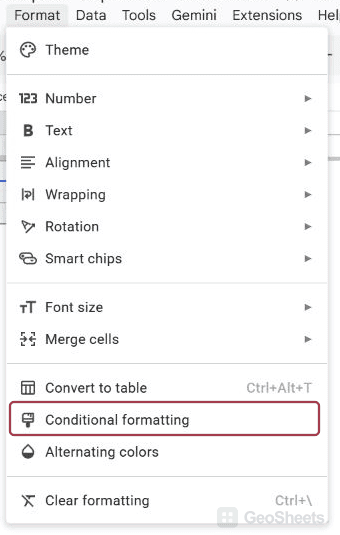
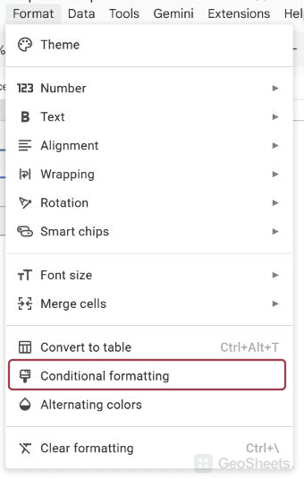
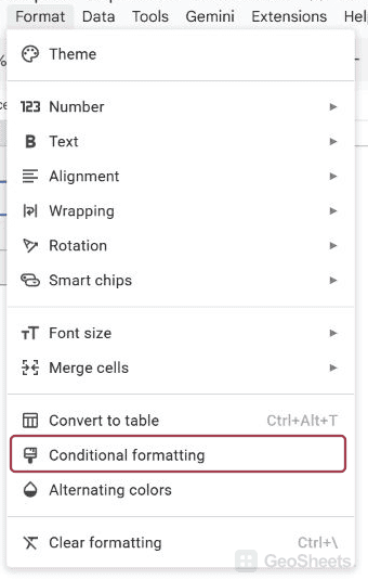
2. Go to Format > Conditional formatting.

   

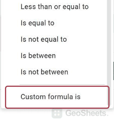
3. Under Format cells if, select Custom formula is.

   

4. Enter the formula below.
5. Choose a fill color and click Done.

=INDIRECT("'Sheet2'!A"&ROW())=TRUE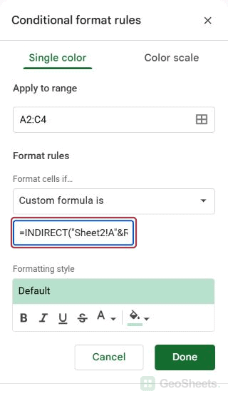

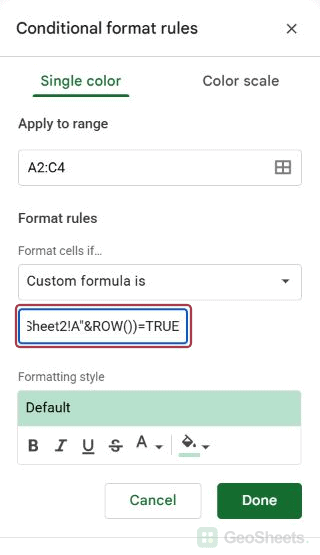
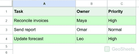
Rows 2 and 4 change color across columns A:C. Row 3 stays unfilled because Sheet2!A3 contains FALSE.

For row 2, ROW() returns 2. Joining it to "'Sheet2'!A" produces the text 'Sheet2'!A2. INDIRECT turns that text into the cell reference we need.

On row 4, the same rule reads Sheet2!A4 instead. That’s why one formula can handle every row in the selected area.

Try changing Sheet2!A3 from FALSE to TRUE. The Send report row should then change color, without editing the formatting rule.

Google’s conditional-formatting instructions specify INDIRECT for cross-tab references in custom rules. A normal reference to another tab isn’t the documented approach inside this rule box.

Keep corresponding records on matching rows

This method connects positions, not task names. Sheet1 row 2 always reads Sheet2 row 2. If someone independently sorts one tab, those rows may no longer describe the same task.

For lists that can be sorted separately, use the ID-based method later in this article. It looks for a matching record instead of assuming the row numbers still correspond.

If your task list begins at row 2 but its flags begin at row 5, there’s a fixed three-row offset. In this captured example, the source tab is named R32022 Sheet2. Apply this version to the task range, and substitute your own tab name if it differs:

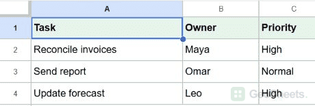
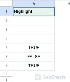
Here are the steps to apply the same matching-row rule when the source flags start three rows lower.

1. Select A2:C4 on the task tab.

   

2. Choose Format > Conditional formatting.

   

3. Choose Custom formula is, then enter the formula below, choose a fill color, and click Done.

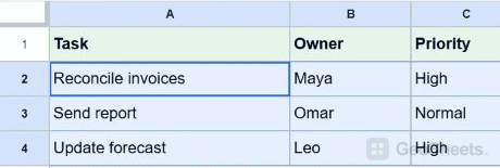
=INDIRECT("'R32022 Sheet2'!A"&(ROW()+3))=TRUE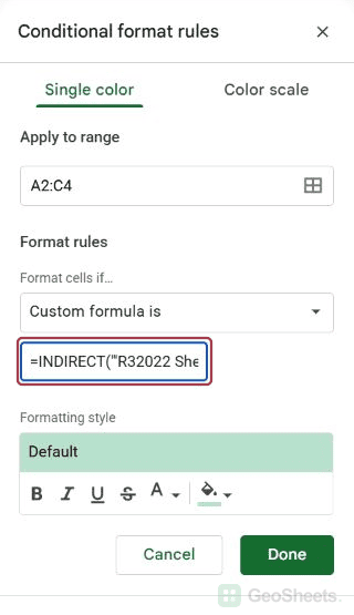

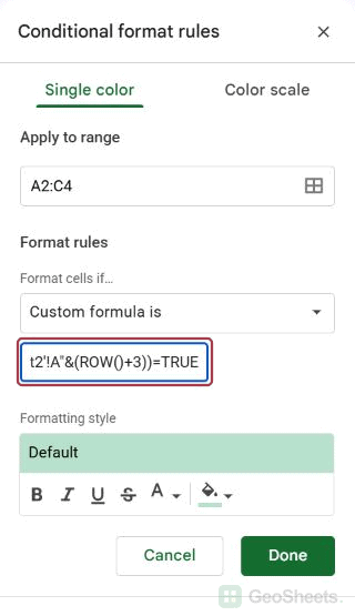
Task row 2 now reads A5, row 3 reads A6, and row 4 reads A7. The lists must still stay in the same order.

Reference a tab whose name contains spaces

Your tabs probably have descriptive names such as Approval Flags rather than Sheet2. You can use those names too; place single quotation marks around the tab name inside the reference text.

For flags in A2:A4 on a tab named Approval Flags, apply this custom rule to your task rows starting at row 2:

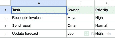
Here are the steps to use a source tab whose name contains spaces.

1. Select A2:C4 on the task tab.

   

2. Choose Format > Conditional formatting.

   

3. Choose Custom formula is, then enter the formula below, choose a fill color, and click Done.

=INDIRECT("'Approval Flags'!A"&ROW())=TRUE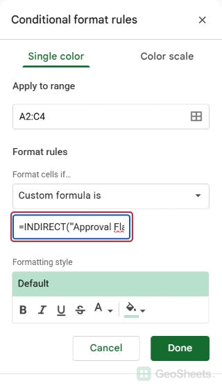

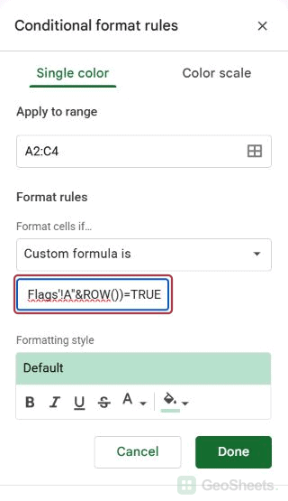
The outer double quotes create the formula’s text string. The inner single quotes surround the tab name. Keep the exclamation mark between the name and the cell address.

To try this variation, create Approval Flags, enter TRUE, FALSE, and TRUE in A2:A4, then replace the earlier rule with this one. The first and third task rows should be highlighted.

Because the tab name sits inside text, remember to update that text if you rename the source tab. The INDIRECT guide explains text-based references in more detail.

Highlight values that meet or exceed a target on another sheet

Suppose you keep a monthly sales target on a Settings tab. You want each salesperson’s revenue highlighted when it reaches that target, and you want to change the target in one place.

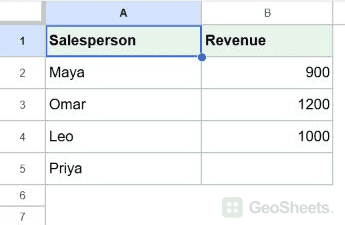
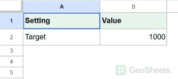
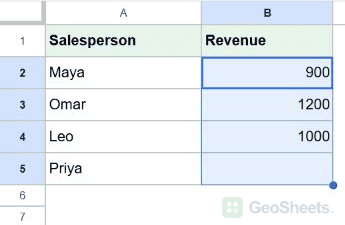
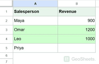
Below, I have names and revenue in A2:B5 on a Sales tab. On Settings, A2 contains Target and B2 contains 1000.

Let’s highlight revenue that meets or exceeds the target.

1. On Sales, select B2:B5.

   

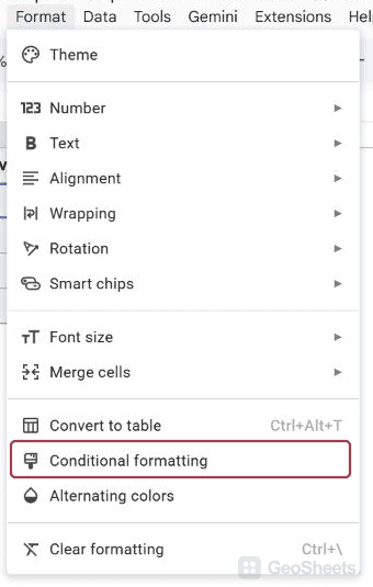
2. Open Format > Conditional formatting and choose Custom formula is.

   

3. Enter the formula below, choose a fill color, and click Done.

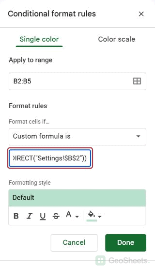
=AND(ISNUMBER(B2),B2>=INDIRECT("Settings!$B$2"))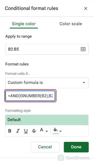

Omar’s 1200 and Leo’s 1000 are highlighted. Maya’s 900 is below target, and Priya’s empty revenue cell stays unfilled.

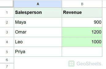
Here, the source reference always points to Settings!B2. We don’t use ROW because every salesperson should be compared with the same target.

ISNUMBER(B2) limits the rule to numeric revenue cells. Enter the target as a number too. Formatting a text entry as currency doesn’t turn it into a usable numeric target.

If you change Settings!B2 to 1100, only Omar’s value qualifies. That makes the target cell useful for reviewing different goals without rewriting the rule.

To highlight the salesperson’s name as well, apply the rule to A2:B5 and use this version:

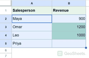
=AND(ISNUMBER($B2),$B2>=INDIRECT("Settings!$B$2"))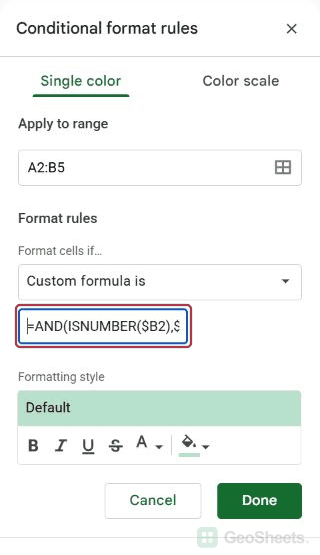

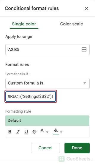
The dollar sign before B makes both cells in each row check the revenue column. Without it, the comparison could move to a different column as the rule runs across the row.

Highlight items that appear in another tab’s list

You may have a customer list on one tab and an approved-customer list on another. Here, the goal is to highlight any customer that appears in the approved list, wherever it appears.

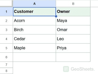
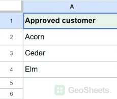
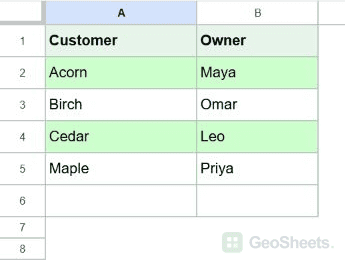
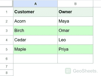
Below, I have customers and owners in A2:B6 on Customers. On a tab named Approved Customers, A2:A4 contains Acorn, Cedar, and Elm.

Here are the steps to highlight approved customers.

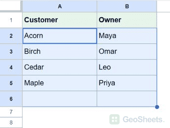
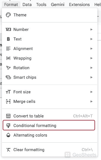
1. On Customers, select A2:B6.

   

2. Open Format > Conditional formatting and select Custom formula is.

   

3. Enter the formula below, choose a fill color, and click Done.

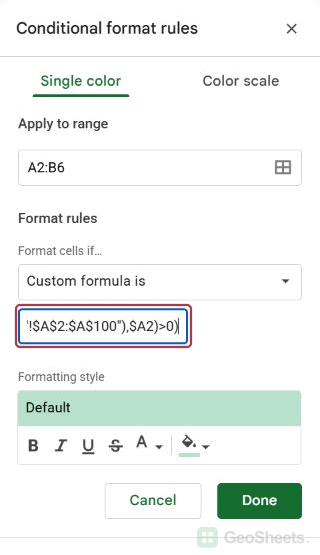
=AND($A2<>"",COUNTIF(INDIRECT("'Approved Customers'!$A$2:$A$100"),$A2)>0)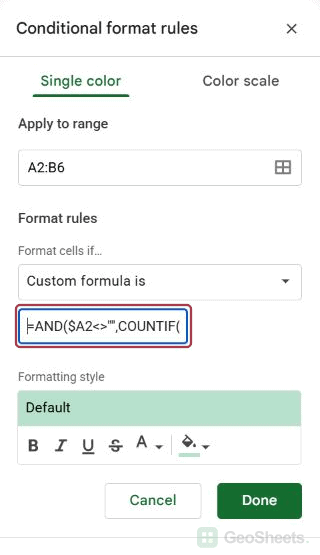

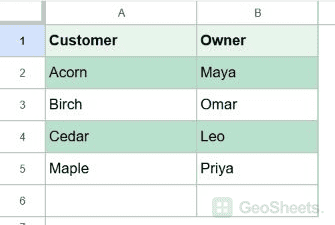
Acorn and Cedar are highlighted across both columns. Birch and Maple aren’t in the approval list, and the empty row stays unfilled.

INDIRECT supplies the other tab’s range. COUNTIF then searches it for the customer in the current row. One match is enough, so we check whether the count is greater than zero.

The search includes rows 2 through 100, allowing room for more approved customers. If you extend the source beyond row 100, extend this reference too.

Unlike the first method, the row order doesn’t need to match. Acorn can be in row 20 of the approval list and still highlight Acorn in row 2 of Customers.

For the opposite result, replace >0 with =0:

=AND($A2<>"",COUNTIF(INDIRECT("'Approved Customers'!$A$2:$A$100"),$A2)=0)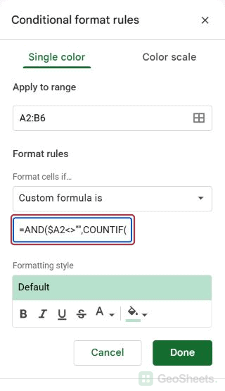

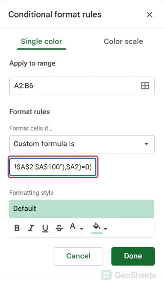
That highlights Birch and Maple as customers missing from the approved list. Keep the blank check so spare rows don’t look like missing customers.

COUNTIF ignores letter case. These examples use ordinary customer names; names containing literal asterisks or question marks need special handling, as explained in the duplicate-highlighting guide.

Match an ID and check its status on another sheet

Finding an ID on another tab isn’t always enough. You might want to highlight an invoice only when that invoice has a Paid status, even after the payment list is sorted.

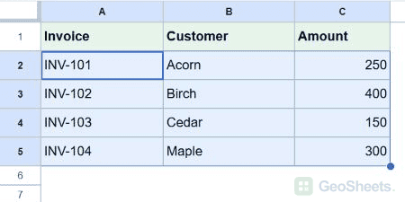
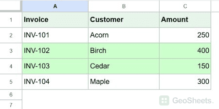
Below, I have invoices in A2:C5 on Invoices. The Payments tab contains invoice IDs in column A and their payment statuses in B, in a different order.

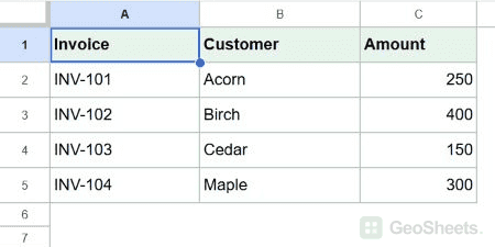
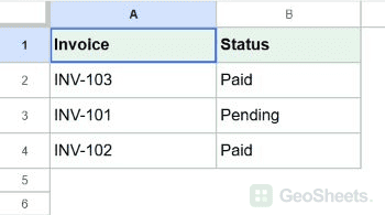
Let’s highlight invoice rows with a matching Paid record.

1. On Invoices, select A2:C5.

   

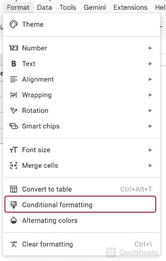
2. Open Format > Conditional formatting and select Custom formula is.

   

3. Enter the following formula, choose a fill color, and click Done.

=AND($A2<>"",COUNTIFS(INDIRECT("Payments!$A$2:$A$100"),$A2,INDIRECT("Payments!$B$2:$B$100"),"Paid")>0)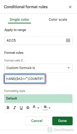

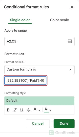
INV-102 and INV-103 are highlighted. INV-101 is Pending, and INV-104 has no matching payment record, so neither receives the fill.

COUNTIFS checks both conditions on the same source row: the invoice ID must match, and the status must be Paid. Both source ranges therefore cover the same rows.

This rule means “at least one matching Paid record exists.” If Payments contains conflicting statuses for the same invoice, it will still highlight an invoice with any Paid match.

For a current-status list, keep one authoritative status per invoice. If you’re storing a payment history instead, decide which entry represents the latest status before building the highlighting rule.

Use data from a separate spreadsheet file

The previous methods read tabs inside the same file. If your approval list lives in a different spreadsheet with its own URL, INDIRECT alone won’t retrieve that data.

A practical approach is to bring the source list into a spare area of your destination sheet with IMPORTRANGE, then point the formatting rule at that local copy.

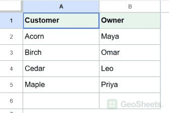
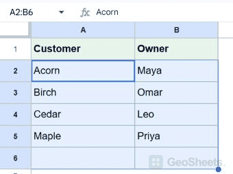
For example, suppose Customers has names in A2:B6, and the separate file has approved names on a tab named Approved, starting at A2.

Here are the steps to connect that list.

1. On Customers, make sure H2:H100 is empty.

   

2. Enter the import formula below in H2, replacing the placeholder with the source spreadsheet URL.
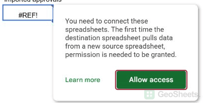
3. If Sheets asks you to connect the files, click Allow access. You need access to the source spreadsheet.

   

4. Wait for the customer names to appear in column H.
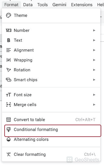
5. Select A2:B6 and create a Custom formula is conditional-formatting rule using the second formula below.

   

   

6. Choose a fill color and click Done.

=IMPORTRANGE("SOURCE_SPREADSHEET_URL","Approved!A2:A100")

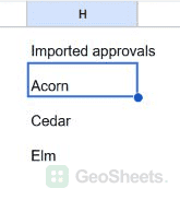
Once the imported list appears, use this formatting rule:

=AND($A2<>"",COUNTIF($H$2:$H$100,$A2)>0)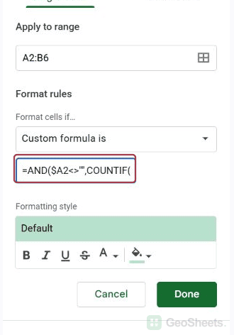

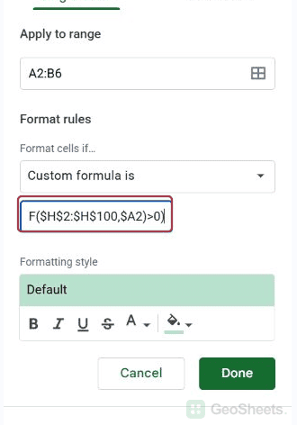
The rule now checks local cells in H. You can hide column H after setting it up, but leave its import formula and output area intact.

Importing creates a data connection, and updates can take time. If the import shows an error or needs permission, fix that connection before expecting the highlighting to reflect the source.

Google’s IMPORTRANGE documentation explains access and refresh behavior. For a full import walkthrough, see the IMPORTRANGE function guide.

Other Google Sheets articles you may also like

• INDIRECT Function in Google Sheets
• Highlight a Row Based on Another Cell
• ROW Function in Google Sheets