Highlight Duplicate Values in Google Sheets

When you’re checking a list of customers, projects, or invoice numbers, repeated entries can be hard to spot. Highlighting them lets you review the matches without deleting anything from your sheet.

In this tutorial, I’ll show you how to highlight duplicates in one column, compare two lists, and find repeated values or complete records across multiple columns.

We’ll use conditional formatting so the highlighting changes when you edit your data. I’ll also show you how to leave the first occurrence alone and keep empty cells out of the results.

Highlight every duplicate value in a column

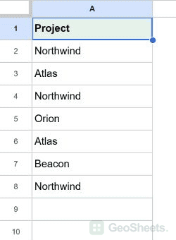
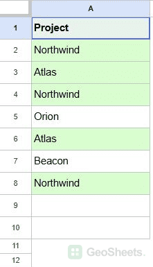
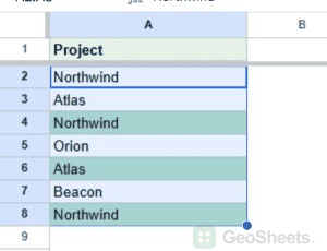
Below, I have a list of projects in A2:A8. Northwind appears three times and Atlas appears twice. I want to highlight every occurrence of those names, including the first one.

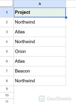
Let’s create a rule that counts how often each name appears in this list.

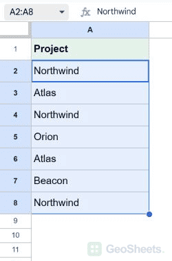
1. Select A2:A8, leaving out the Project heading.

   

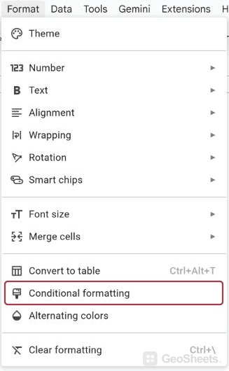
2. Go to Format > Conditional formatting.

   

3. Under Format cells if, select Custom formula is.

   

4. Enter the formula below.
5. Choose a fill color under Formatting style, then click Done.

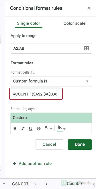
=COUNTIF($A$2:$A$8,A2)>1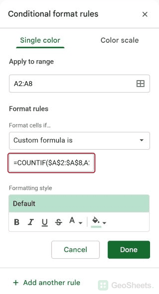

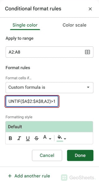
This highlights A2, A3, A4, A6, and A8. Orion and Beacon stay unfilled because each appears only once.

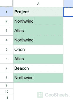
The COUNTIF function counts matches for the current cell. For A2, it counts Northwind three times. Since three is greater than one, that cell gets highlighted.

The dollar signs in $A$2:$A$8 keep the search area fixed. The reference A2 changes as the rule moves down, so each project gets its own comparison.

If you’re using a longer list, replace $A$8 with its last cell and update Apply to range as well. Changing only one can leave part of your list unchecked.

Keep blank cells out of the highlighting

Your real list may include empty rows or space for future entries. In that case, I’d add a check that the current cell isn’t empty.

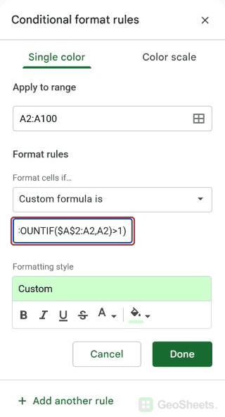
For a list that can grow through row 100, select A2:A100 and use this custom formula:

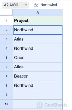
=AND(A2<>"",COUNTIF($A$2:$A$100,A2)>1)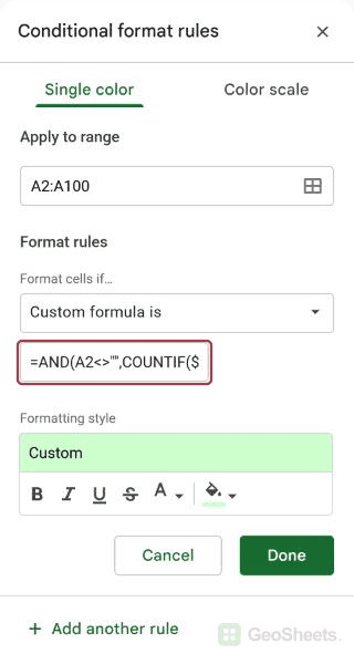

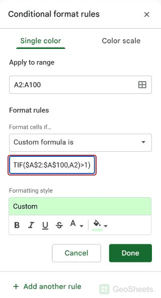
The first condition excludes empty cells, including formulas that return an empty string. The second condition still checks for duplicates. A space character isn’t empty, so clean stray spaces from your data separately.

Google’s COUNTIF documentation specifies case-insensitive matching. That means Atlas and ATLAS count as the same name in these examples.

Highlight only the second and later occurrences

Sometimes you want to keep the first entry and review only the copies that come after it. For the project list above, that means leaving the first Northwind and Atlas unfilled.

We’ll still compare the project names in A2:A8, but this time we’ll count only from the beginning of the list down to the current row.

Here are the steps to highlight later occurrences.

1. Select A2:A8 and open Format > Conditional formatting.

   

   

2. Click the existing duplicate rule to replace it, or create a rule if this range doesn’t have one.
3. Choose Custom formula is and enter the formula below.
4. Choose a fill color and click Done.

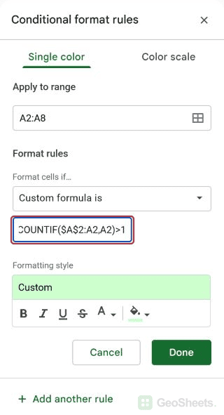
=COUNTIF($A$2:A2,A2)>1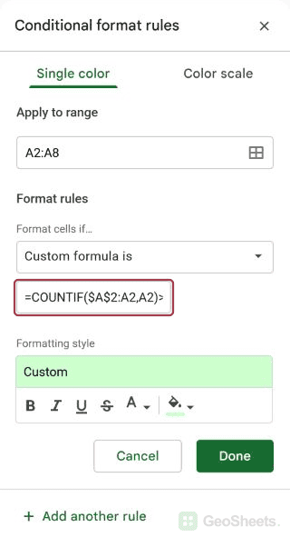

Now A4, A6, and A8 are highlighted. The first Northwind in A2 and the first Atlas in A3 remain unfilled.

In row 2, the range is just A2:A2. By row 4, it has expanded to A2:A4, so the second Northwind has a count of two.

Notice that only the beginning, $A$2, is fully locked. The end of the range moves down one row at a time. That’s what makes this different from the first formula.

If you allow empty rows through row 100, apply the following version to A2:A100:

=AND(A2<>"",COUNTIF($A$2:A2,A2)>1)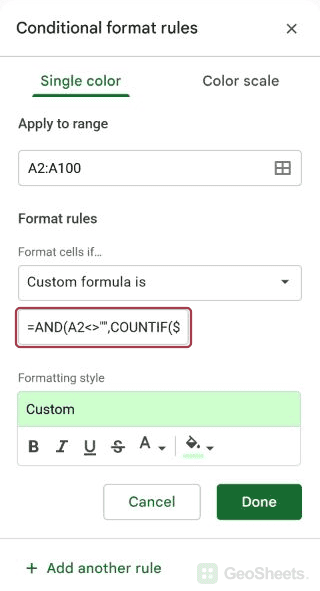

“First” means the earliest occurrence in the current row order. If you sort the list, a different record may become the first one. Highlighting doesn’t decide which record you should delete.

Highlight repeated values anywhere in multiple columns

Suppose three teams have entered project names in separate columns. You want to see which projects appear more than once anywhere in the combined area, regardless of the team or row.

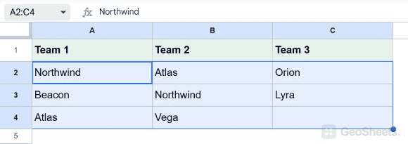
Below, I have the team lists in A2:C4.

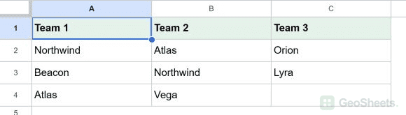
Let’s check all three columns as one group.

1. Select A2:C4.

   

2. Open Format > Conditional formatting and choose Custom formula is.

   

3. Enter the formula below, choose a fill color, and click Done.

=AND(A2<>"",COUNTIF($A$2:$C$4,A2)>1)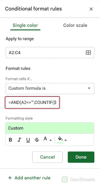

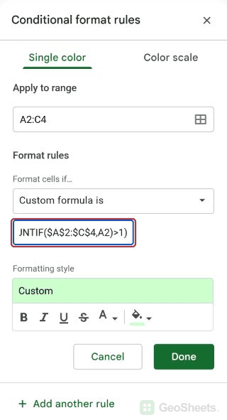
Northwind in A2 and B3 is highlighted, along with Atlas in B2 and A4. The blank cell in C4 stays unfilled.

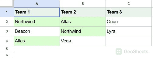
Here, $A$2:$C$4 covers the entire comparison area. The unlocked A2 can move across columns as well as down rows, letting each cell supply its own project name.

Don’t change that reference to $A2 for this method. Locking column A would make the other columns depend on the project in A rather than their own contents.

This finds repeated individual values. If your columns contain different fields, such as customer, product, and quantity, use the complete-record method below instead.

Compare two lists and highlight the matches

You may have an existing project list and a second list of proposed projects. Here, you want to highlight proposed names that already exist, even if a proposed name appears only once.

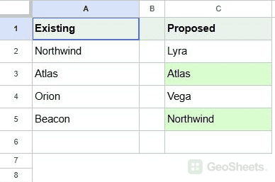
Below, I have existing projects in A2:A5 and proposed projects in C2:C6.

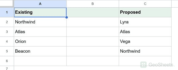
Let’s highlight matches in the proposed list.

1. Select C2:C6.

   

2. Open Format > Conditional formatting and select Custom formula is.

   

3. Enter the formula below, select a fill color, and click Done.

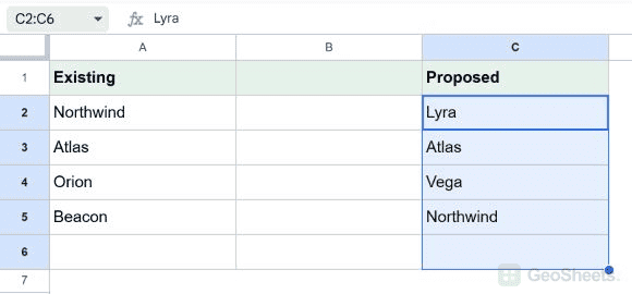
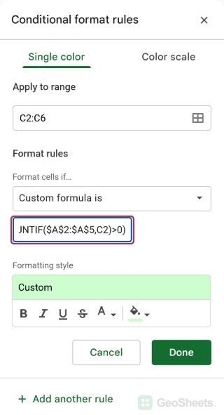
=AND(C2<>"",COUNTIF($A$2:$A$5,C2)>0)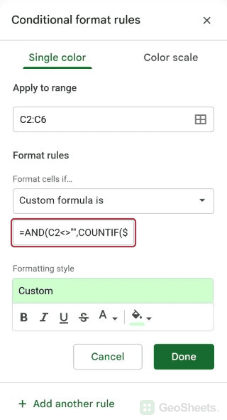

C3 and C5 are highlighted because Atlas and Northwind appear in the existing list. Lyra and Vega aren’t highlighted, and the blank at the bottom is excluded.

We use >0 here because one match in the other list is enough. The proposed cell itself isn’t part of the range we’re counting.

This compares each proposed project against the whole existing list. It doesn’t require matching names to be on the same row.

To color matching names in the existing list too, create a separate rule for A2:A5:

=AND(A2<>"",COUNTIF($C$2:$C$6,A2)>0)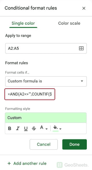

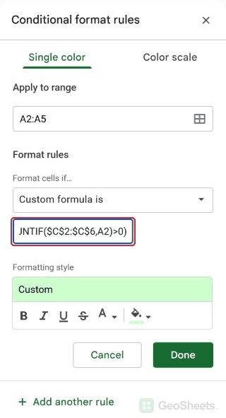
That highlights A2 and A3. If the comparison list is on another tab, see conditional formatting across sheets for the cross-tab reference setup.

Highlight entire rows with a duplicate ID

If you’re reviewing invoices, highlighting the whole row can make the amount and customer easier to compare. The duplicate check can still depend on just the invoice number.

Below, I have invoice IDs in column A, customers in B, and amounts in C. I want every row with a repeated invoice ID to stand out.

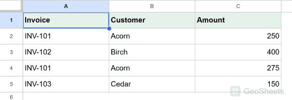
Here are the steps to color the full invoice records.

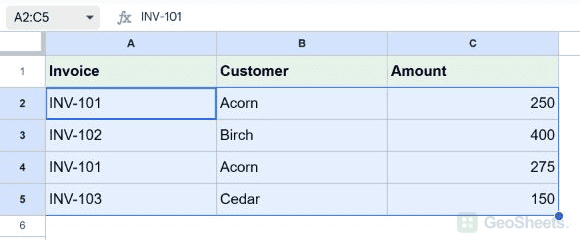
1. Select A2:C5, including the customer and amount columns.

   

2. Open Format > Conditional formatting and choose Custom formula is.

   

3. Enter the formula below, select a fill color, and click Done.

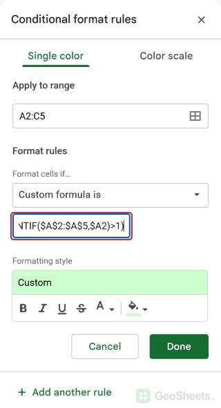
=AND($A2<>"",COUNTIF($A$2:$A$5,$A2)>1)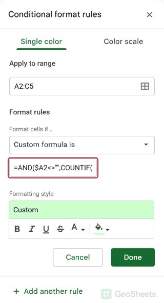

Rows 2 and 4 are highlighted across A:C. Their amounts differ, but their invoice IDs match. That’s useful when you’re checking whether an invoice was entered twice with inconsistent details.

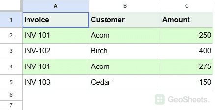
The $A2 reference keeps every cell in a row looking at column A. The row number can still change, so row 4 checks A4 rather than A2.

If your ID is in B instead, change both the count range and the current-cell reference to column B. Keep the applied range wide enough to include every field you want colored.

Highlight complete duplicate records

A repeated customer name doesn’t necessarily mean a duplicate order. You may want a match only when the customer, product, and quantity are all identical.

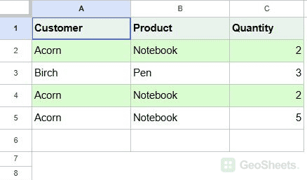
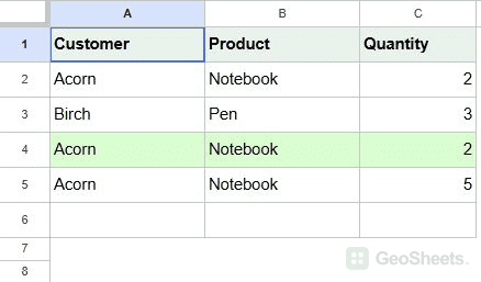
Below, I have order details in A2:C6. Acorn ordered notebooks twice in the same quantity, but its notebook order for five units should remain separate.

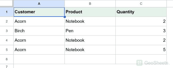
Let’s check the three fields together.

1. Select A2:C6.

   

2. Open Format > Conditional formatting and select Custom formula is.

   

3. Enter the formula below, choose a fill color, and click Done.

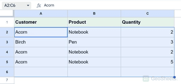
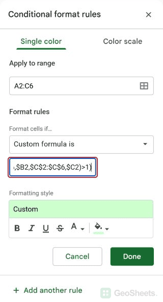
=AND($A2<>"",COUNTIFS($A$2:$A$6,$A2,$B$2:$B$6,$B2,$C$2:$C$6,$C2)>1)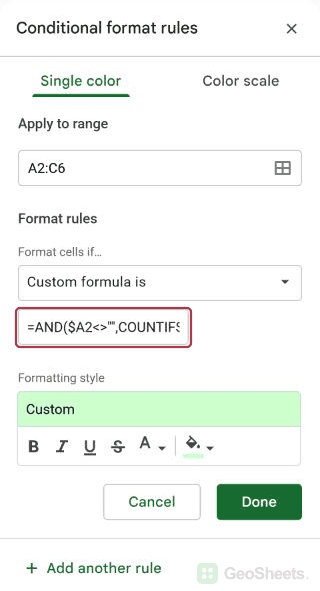

Rows 2 and 4 are highlighted. Row 5 stays unfilled because its quantity is different. The empty row is excluded because its customer cell is blank.

COUNTIFS counts rows where all three field comparisons match. Checking fields separately also avoids confusing records that happen to produce the same text when joined together.

Use a required field for the blank check. Here, every genuine order needs a customer in A. If your records can legitimately have a blank customer, check a required order ID instead.

To highlight only later copies of a complete record, apply this version to A2:C6:

=AND($A2<>"",COUNTIFS($A$2:$A2,$A2,$B$2:$B2,$B2,$C$2:$C2,$C2)>1)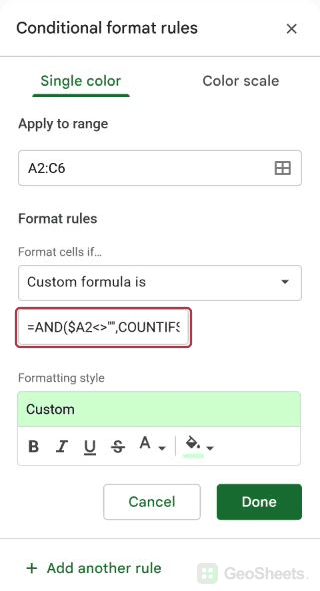

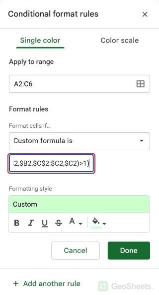
Only row 4 is highlighted. Each comparison range expands to the current row, so the first matching record is left alone.

Handle names or codes containing * and ?

If your codes contain an asterisk or question mark, the basic COUNTIF formulas need an adjustment. Those characters have special matching meanings and can match other text.

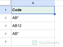
For example, a code of AB* shouldn’t automatically count AB12 as a duplicate. We can compare the cell values directly so those characters are treated as part of the code.

For text codes in A2:A100, use this custom rule:

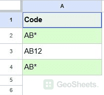
1. Enter AB*, AB12, and AB* in A2:A4, then select A2:A100.

   

2. Choose Format > Conditional formatting and set Format cells if to Custom formula is.

   

3. Enter the formula below, choose a fill color, and click Done.

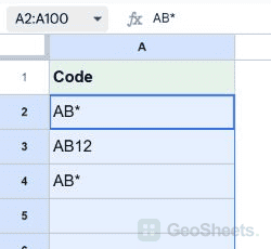
=AND(A2<>"",SUMPRODUCT(--($A$2:$A$100=A2))>1)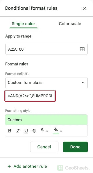

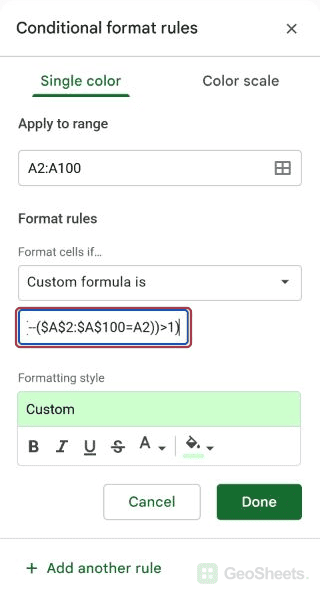
The comparison checks each cell against the current code. The double minus converts the matches to ones and the nonmatches to zeros; SUMPRODUCT adds them to count matching codes.

If A2:A4 contains AB*, AB12, and AB*, only A2 and A4 should be highlighted with this rule. Use it for literal text codes rather than changing the simpler project-name examples unnecessarily.

Other Google Sheets articles you may also like

• COUNTIF Function in Google Sheets
• Absolute References in Google Sheets
• Highlight a Row Based on Another Cell