
When one choice determines the next, a regular dropdown isn’t enough. You might want an Item menu that shows fruit only when the Category cell says Fruit.
I’ll show you how to keep the categories and items on a separate tab, filter the items into a helper range, and use that range for the second dropdown.
Set up the categories and items
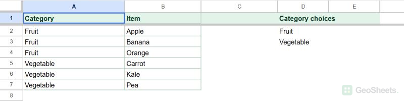
Name the source tab GSN012 Lists. Columns A and B pair each item with its category. D2:D3 holds one copy of each category for the first dropdown.
Name the working tab GSN012 Orders. It starts with one order in A2. Category in B2 and Item in C2 are empty. Filtered items will appear in G2:G7.
Use these tab names if you want to paste the formula exactly. If your tabs have different names, replace the quoted names in the formula and validation ranges.

Create the first dropdown for Category
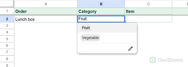
First, let’s make B2 offer the two categories from GSN012 Lists.
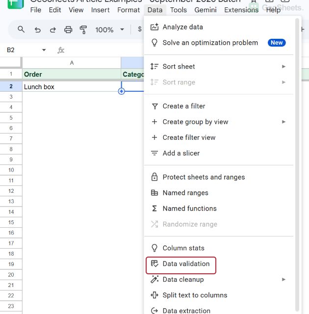
1. Select GSN012 Orders!B2, then choose Data > Data validation.
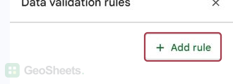
2. In the rules sidebar, click Add rule if no new rule is open.
3. Set Apply to range to B2. Under Criteria, choose Dropdown from a range and select ‘GSN012 Lists’!$D$2:$D$3.
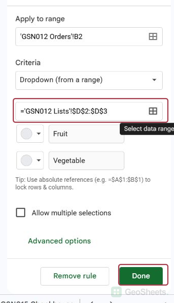
4. Click Done. Choose Fruit in B2, then reopen it to check both category choices.
Filter the items for the chosen category
We now need a short list that changes with B2. Put this formula in GSN012 Orders!G2, leaving the cells below it empty so the results can expand.
=FILTER('GSN012 Lists'!$B$2:$B$7,'GSN012 Lists'!$A$2:$A$7=$B$2)
The first range supplies items. The second checks their categories against B2. With Fruit selected, the helper should contain Apple, Banana, and Orange.
If G2 shows #N/A, check that B2 contains a category used in ‘GSN012 Lists’!A2:A7. Google Sheets returns this error when FILTER finds no matching rows.
If the formula cannot expand, clear any values in G3:G7.
Use the filtered range for the Item dropdown
Here are the steps to use the helper values as C2’s choices.
1. Select GSN012 Orders!C2, open Data > Data validation, and add a rule for C2.
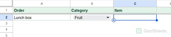
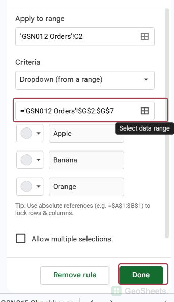
2. Choose Dropdown from a range. Set its source to the helper cells ‘GSN012 Orders’!$G$2:$G$7, then click Done.
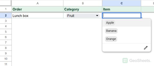
3. Open C2. Check that its choices match the three Fruit items in G2:G4, then choose Apple.
To check the dependency, change B2 to Vegetable. The old Item can remain in C2 even though it no longer belongs to the category. In this example, Sheets marks Apple invalid.
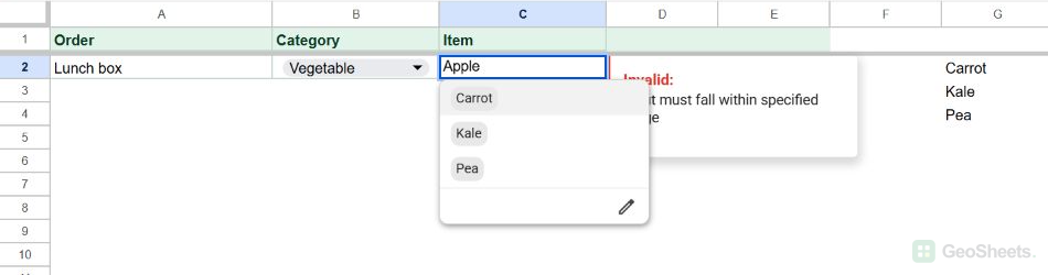
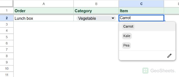
Open C2 and choose a valid item. Its choices now match Carrot, Kale, and Pea in the helper range.
When your source is in another place
This example stores the source on another tab in the same spreadsheet. If your categories are in a different spreadsheet file, first bring that data into this file with IMPORTRANGE.
You can then build the helper and dropdown from local cells. If you only need one unchanged list from another tab, use a dropdown rule that points directly to that range.
Other Google Sheets articles you may also like