
When you’re working with sales figures, scores, or expenses in Google Sheets, you may want to quickly spot the highest or lowest value without scanning every number.
Conditional formatting can highlight those values for you. If a number changes, the highlighting changes with it, so you don’t have to keep recoloring cells yourself.
In this tutorial, I’ll show you how to highlight the highest and lowest values in a list, compare numbers within each row or column, and highlight a top or bottom group.
Highlight the highest value in a column
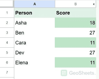
Let’s start with a short list of scores. Below, I have five people in column A and their scores in B2:B6. I want to make the highest score easy to find.
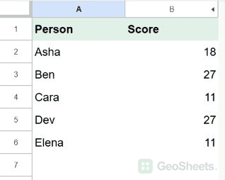
You can use your own list instead. Keep the column heading outside the selection, and note the first and last cells containing your scores.
Here are the steps to highlight the highest score:
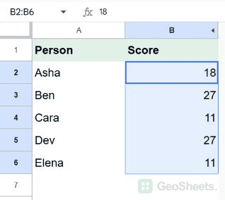
- Select B2:B6.

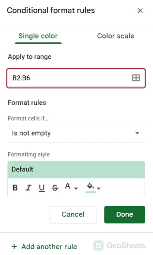
- Click Format > Conditional formatting.

- In the sidebar, check that Apply to range is B2:B6.

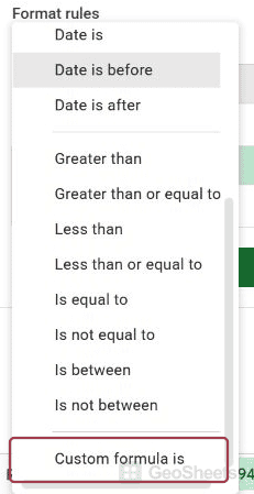
- Under Format cells if, choose Custom formula is.

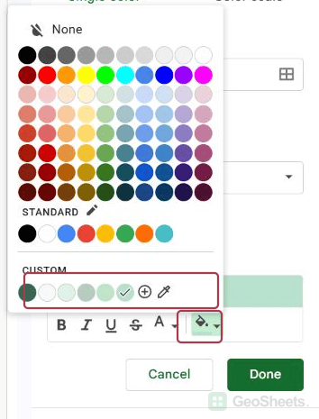
- Enter the formula below, choose a green fill under Formatting style, and click Done.


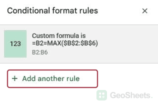
=B2=MAX($B$2:$B$6)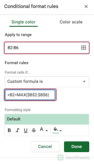
Both cells containing 27, B3 and B5, get highlighted. That’s useful when two people share the highest score: you don’t have to choose just one of them.
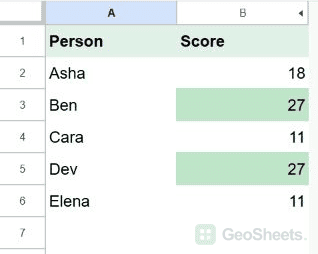
Here’s what the formula is doing. MAX($B$2:$B$6) finds the largest score, 27. Sheets then asks whether each cell in your selected range equals that number.
The first B2 changes as Sheets checks each score. The dollar signs keep $B$2:$B$6 fixed, so every person is compared against the same complete list.
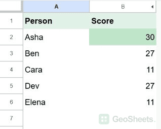
If you change Asha’s score from 18 to 30, Asha’s score becomes the highlighted maximum. Ben and Dev no longer meet the rule.
Highlight the lowest value in a column
Now let’s highlight the lowest score in that same list. With 18, 27, 11, 27, and 11 in B2:B6, the lowest value is 11.
You can keep the highest-value rule and add a second color for the lowest value. If you only want the minimum, you can create this rule on its own.
Here are the steps to add the lowest-score highlight:
- Select B2:B6 and open Format > Conditional formatting.
- Click Add another rule if your highest-score rule is already there.

- Set Apply to range to B2:B6 and choose Custom formula is.

- Enter the formula below.
- Choose a different fill, such as pale orange, and click Done.
=B2=MIN($B$2:$B$6)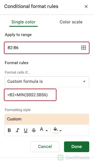
Cells B4 and B6 now receive the lowest-score color. The formula works like the previous one, but MIN finds the smallest number in the list.
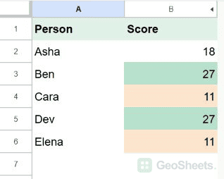
Both formulas include ties. If every score is identical, every score is both the highest and lowest. When the rules overlap, the first matching rule in the sidebar determines the format.
You can drag the rule you want to take priority above the other one. For example, put the highest-score rule first if equal scores should appear green.
Use the formulas with a different range
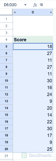
Suppose your numbers are in D5:D20 instead. Your selected range, the first cell in the formula, and the fixed comparison range all need to refer to that list.
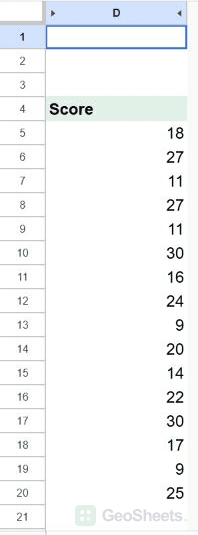
Here are example scores in D5:D20. Select that range before creating either rule.
For the highest number in D5:D20, use:
=D5=MAX($D$5:$D$20)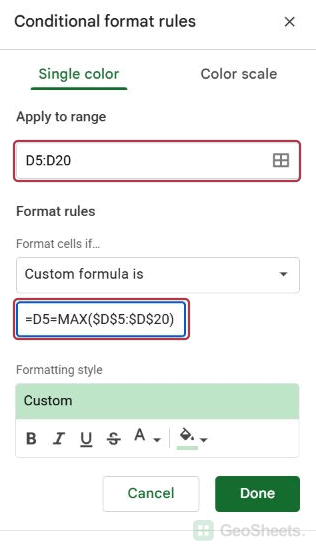
For the lowest number in D5:D20, use:
=D5=MIN($D$5:$D$20)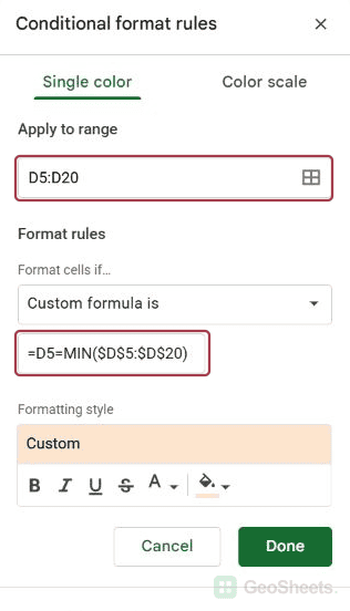
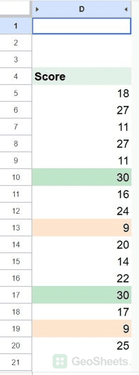
Starting the formula at D2 while the selection starts at D5 would check the wrong row. Matching that first reference is just as important as changing the range inside MAX or MIN.
Highlight the entire row containing the highest or lowest value
Sometimes the number alone isn’t enough. In our score list, you may want the person’s name highlighted too, so you can immediately see who achieved the highest score.
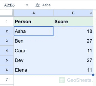
For this example, names are in A2:A6 and scores are in B2:B6. We’ll color both cells in each matching record.
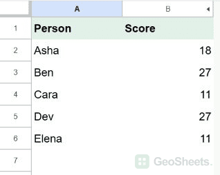
Here are the steps to highlight the whole record:
- Select A2:B6, including the names and scores.
- Open Format > Conditional formatting.
- Create a rule with Custom formula is.
- Enter the formula below, choose a fill color, and click Done.
=AND(ISNUMBER($B2),$B2=MAX($B$2:$B$6))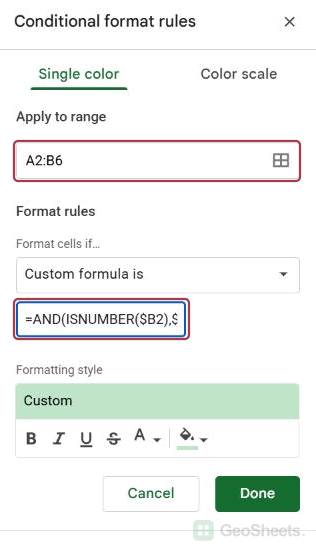
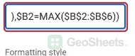
Ben’s and Dev’s records, A3:B3 and A5:B5, are highlighted. ISNUMBER ensures the score is a number, while the second condition checks whether it is the maximum.
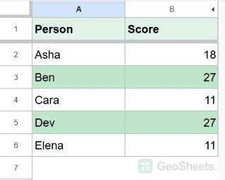
Notice the extra dollar sign in $B2. It keeps every cell in the record looking at column B, even while the formatting extends across column A.
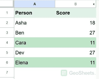
To highlight the records with the lowest score instead, use this formula with the same A2:B6 selection:
=AND(ISNUMBER($B2),$B2=MIN($B$2:$B$6))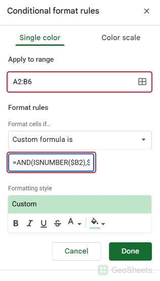
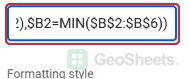
That highlights Cara’s and Elena’s records. If your table has more columns, expand Apply to range to include them while keeping the score reference locked to column B.
For other conditions that can color a complete record, see highlighting an entire row based on another cell.
Highlight the highest and lowest value in each row
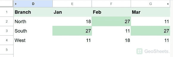
Let’s look at a different layout. Below, each branch has three monthly totals. I want to identify each branch’s best month, rather than find one maximum for the entire table.
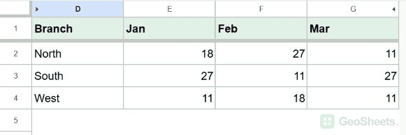
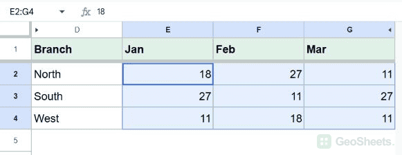
Here are the steps to compare the months within each row:
- Select the numeric area, E2:G4.

- Open Format > Conditional formatting and choose Custom formula is.
- Enter the formula below, choose a fill color, and click Done.
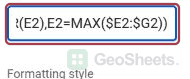
=AND(ISNUMBER(E2),E2=MAX($E2:$G2))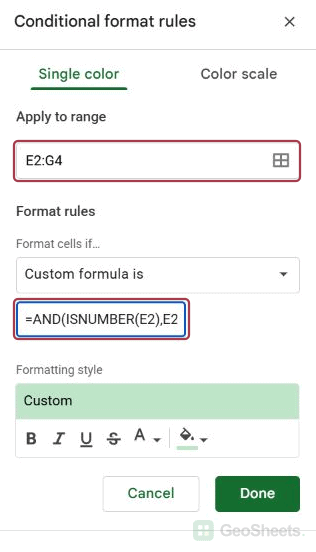
North’s February total is highlighted. South has a tie between January and March, so both are highlighted. West’s February total is its highest value.
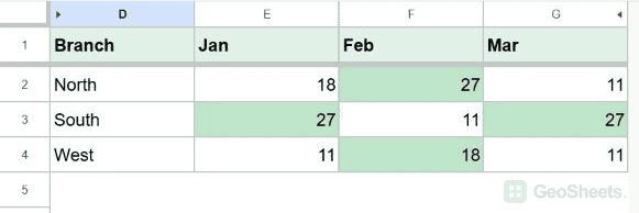
The range $E2:$G2 stays between columns E and G, but its row number can change. That lets Sheets compare row 2 with row 2, row 3 with row 3, and so on.
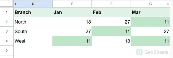
To highlight each branch’s lowest month instead, replace the maximum rule for E2:G4 with:
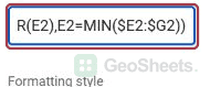
=AND(ISNUMBER(E2),E2=MIN($E2:$G2))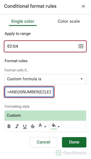
This highlights March for North, February for South, and both January and March for West. Again, tied values all qualify.
Highlight the highest and lowest value in each column
Using the branch table in D1:G4, you might instead want to know which branch performed best each month. Now we need to compare down each column.
The selection is still E2:G4, but the dollar signs move. We’ll fix the row boundaries and let the column change.
If you tried the row-by-row example on this table, remove those rules first. Otherwise, their highlights can hide the results of the new column comparisons.
Here are the steps to highlight each month’s highest total:
- Select E2:G4 and open Format > Conditional formatting.
- Create a Custom formula is rule using the formula below.
- Choose a fill color and click Done.
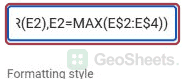
=AND(ISNUMBER(E2),E2=MAX(E$2:E$4))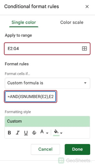
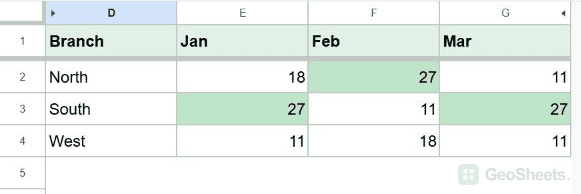
South has the highest January total, North has the highest February total, and South has the highest March total. Those are cells E3, F2, and G3.
In E$2:E$4, rows 2 and 4 stay fixed. The column can move to F or G, so each month’s figures get their own comparison.
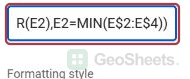
To highlight the lowest total in each month instead, replace the maximum rule for E2:G4 with:
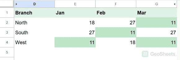
=AND(ISNUMBER(E2),E2=MIN(E$2:E$4))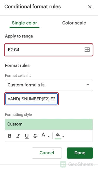
This highlights West in January, South in February, and both North and West in March.
If you want one maximum across the entire table instead, fix both the rows and columns of the comparison range:
=AND(ISNUMBER(E2),E2=MAX($E$2:$G$4))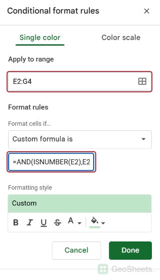
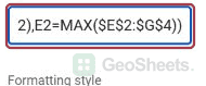
With that rule applied to E2:G4, every 27 qualifies. You can replace MAX with MIN to find the overall minimum instead.
Keep blank cells out of the highlighting
Your real list may have missing entries or labels such as Pending. The basic MAX and MIN calculations ignore nonnumeric cells in the referenced range, but the comparison also needs to exclude blank cells.
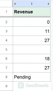
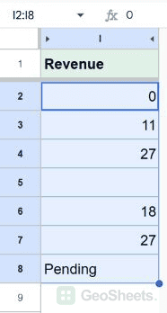
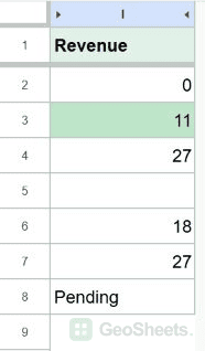
Let’s say I have 0, 11, 27, a blank, 18, 27, and Pending in I2:I8. I want the lowest numeric value, including a genuine zero.
For that list, select I2:I8 and create a custom rule using:
=AND(ISNUMBER(I2),I2=MIN($I$2:$I$8))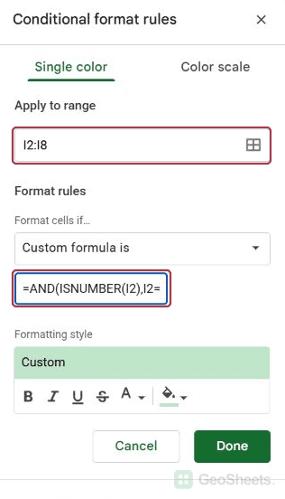
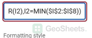
Only I2, containing zero, qualifies. The ISNUMBER(I2) check prevents the blank or Pending entry from receiving the same formatting.
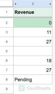
You can use the same safeguard with MAX. It’s particularly useful when your rule covers space for future entries or when a formula returns an empty string.
A number stored as text also fails ISNUMBER. If an imported score looks numeric but is skipped, check its actual value before changing the highlighting rule.
Ignore zeros when finding the lowest value
Sometimes zero means “not entered yet” in your data. If that’s how your list works, you can exclude zeros from the minimum comparison.
For the same I2:I8 list, use:
=AND(ISNUMBER(I2),I2<>0,I2=MINIFS($I$2:$I$8,$I$2:$I$8,"<>0"))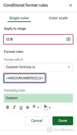
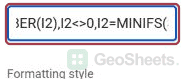
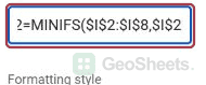
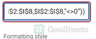
Now the 11 in I3 is highlighted. MINIFS finds the smallest value satisfying a condition; here, that condition is “not zero.”
This excludes zero, not negative numbers. If your list contains -5, that value still qualifies as smaller than 11. Only exclude values when that matches what they mean in your data.
Highlight the top three or bottom three values
What if you want a shortlist instead of only the highest score? Let’s return to the five scores in B2:B6: 18, 27, 11, 27, and 11.
We can use LARGE to find the third-largest score, then highlight every score at least that large.
If B2:B6 still has the earlier highest- and lowest-value rules, remove them before trying this example. That lets the top-group rule supply the color for every qualifying score.
Here are the steps to highlight the top three scores:
- Select B2:B6 and open Format > Conditional formatting.
- Create a Custom formula is rule.
- Enter the formula below, choose a fill, and click Done.
=AND(ISNUMBER(B2),B2>=LARGE($B$2:$B$6,3))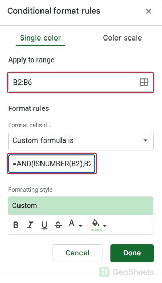
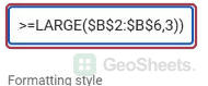
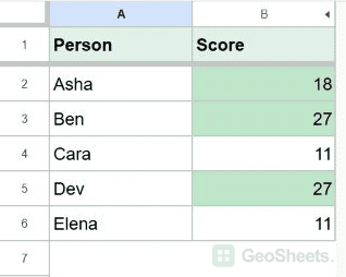
The third-largest score is 18, so B2, B3, and B5 are highlighted. Change the final 3 to 5 if you want the top five in a longer list.
To highlight the bottom three scores, use SMALL and reverse the comparison:
=AND(ISNUMBER(B2),B2<=SMALL($B$2:$B$6,3))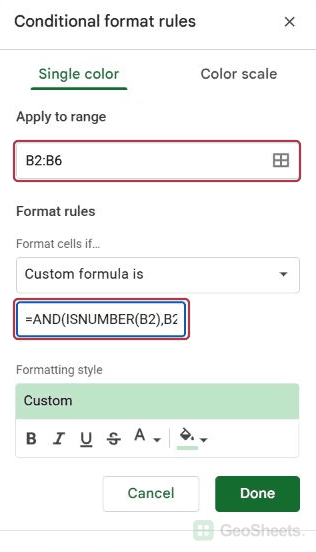
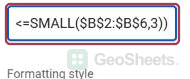
That highlights B2, B4, and B6: the 18 and both 11s. Your chosen group size must not exceed the number of numeric entries in the list.
Ties at the cutoff can highlight more than the requested number of cells. For example, the top two values in 30, 20, 20, and 10 include both 20s, producing three highlighted cells.
That’s usually helpful when equal results should receive equal treatment. If you need ranking numbers alongside your data, our RANK tutorial explains how ties affect those positions.
Other Google Sheets articles you may also like