Fix Conditional Formatting That Is Not Working in Google Sheets

You’ve created a conditional formatting rule, but the cells haven’t changed color. Or perhaps they have changed, just one row away from where you expected.

You don’t necessarily need to start again. A small mismatch between the selected range, the formula, and the values in your cells can explain the result.

In this tutorial, I’ll walk you through specific examples of these problems and their fixes, including skipped rows, unexpected colors, text that looks like numbers, and formulas that refer to another tab.

Find the problem from what you see

Start with the symptom closest to yours. The sections below show you what to inspect and give you a small example to compare against your own sheet.

What you see	What to check
Only one column changes color	The width of Apply to range
The wrong row changes color	The first row referenced in the formula
Every row follows the first row	A dollar sign locking the row number
Matching-looking values are skipped	Spaces, data types, or an error in the condition
The cell has the wrong color	Overlapping rules and their order
Blank-looking cells are highlighted	Empty strings, blanks, and numeric comparisons
A formula from another tab is rejected	Use INDIRECT for the cross-tab reference
New rows don’t receive formatting	The end of Apply to range

When you edit a rule, change one thing at a time. That makes it easier to see which change solves the problem.

Check Apply to range when only some cells are colored

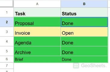
Let’s say you have tasks in column A and their status in column B. You want a completed task’s whole record highlighted.

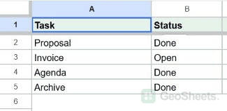
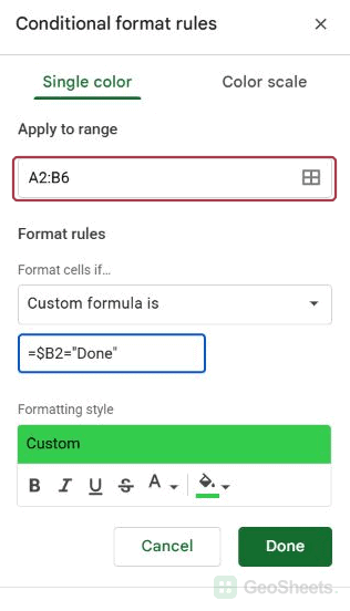
The rule =$B2="Done" can identify the right records. But if Apply to range is B2:B5, it can color only the Status cells.

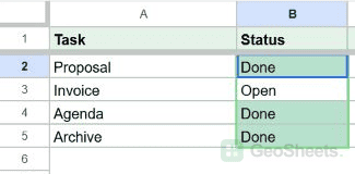
Here are the steps to include the task names too:

1. Select a cell that already has the rule, such as B2.

   

2. Open Format > Conditional formatting.

   

3. Click the relevant rule in the sidebar.
4. Change Apply to range from B2:B5 to A2:B5.

   

5. Keep the custom formula below and click Done.

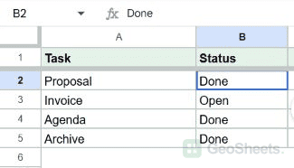
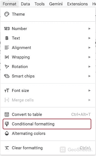
=$B2="Done"

Rows 2, 4, and 5 now have both cells highlighted. The selection controls where the color appears; the formula controls which records qualify.

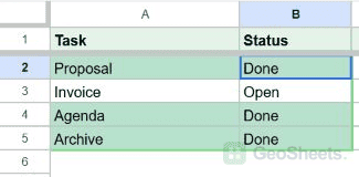
For a wider table, extend the selection across the columns you want colored. Keep $B2 if column B still contains the status you’re checking.

Fix a rule that highlights the wrong row

If the highlighting appears one row below the matching status, compare the formula’s starting row with the first row in Apply to range.

For our task table in A2:B5, the formula needs to start by checking B2. Starting with B1 makes the first data row check the heading instead.

For example, this formula starts too high:

=$B1="Done"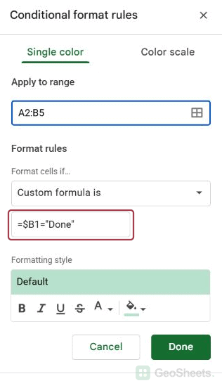

Applied to A2:B5, it highlights rows 3 and 5. Each row is looking at the status above it, which explains why the color appears displaced.

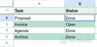
To fix the offset, open the rule and replace it with:

=$B2="Done"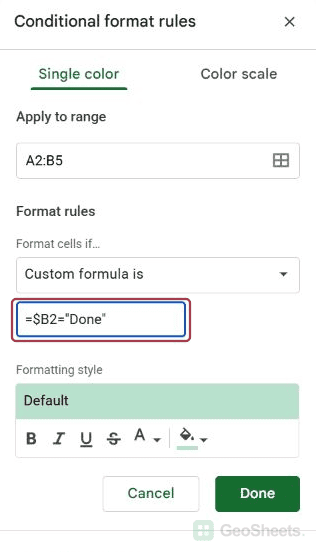

Rows 2, 4, and 5 now match their own status. If your real selection starts at A7, the corresponding formula should begin with $B7.

This follows Google’s instruction to write a custom rule for the first row of its selected range.

Remove a locked row when every record follows the first one

Using the same A2:B5 task table, suppose every record turns green even though Invoice is still Open. A fully locked reference may be the reason.

This formula checks B2 for every cell in the selection:

=$B$2="Done"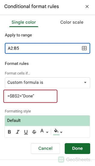

Because B2 contains Done, the condition is true everywhere. Changing any other status has no effect on the result.

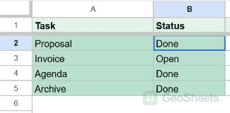
Remove the dollar sign before the row number, leaving the column locked:

=$B2="Done"

Now the rule checks B2 for row 2, B3 for row 3, and so on. The table below puts the three reference patterns side by side.

Formula for A2:B5	Highlighted rows	What it checks
=$B$2="Done"	2, 3, 4, 5	B2 for every record
=$B2="Done"	2, 4, 5	Each record’s own status
=$B1="Done"	3, 5	The status one row above

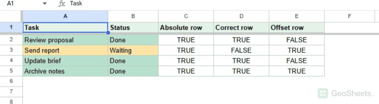
The dollar sign before B still matters. Without it, the reference can move sideways when you color several columns. Our absolute reference guide explains these combinations.

Put the condition in a spare cell to see its result

A rule that doesn’t highlight anything may simply be evaluating to FALSE. Trying the condition in an unused cell lets you see the answer instead of guessing from the color.

For our status example, I’ll use D2 beside the first task. Choose another empty column if D already contains your data.

Here are the steps to inspect the condition:

1. Enter =$B2="Done" in the spare cell on row 2.
2. Copy the formula down through row 5.

   

3. Compare the TRUE and FALSE results with the statuses beside them.
4. If the results are right, inspect the formatting range and rule order. If they’re wrong, inspect the values or formula.

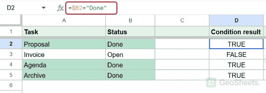
For Done, Open, Done, and Done, the results should be TRUE, FALSE, TRUE, and TRUE. A visible formula error gives you a more specific clue to investigate.

For example, =SEARCH("urgent",B2) returns an error when the word isn’t found. A text-formatting condition can use this instead:

=ISNUMBER(SEARCH("urgent",B2))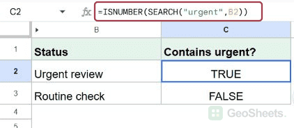

That produces TRUE when urgent is found and FALSE otherwise. It’s useful for text searches, but it won’t repair a misspelled function or an incorrect cell reference.

Check extra spaces when matching text is skipped

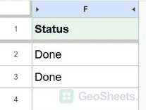
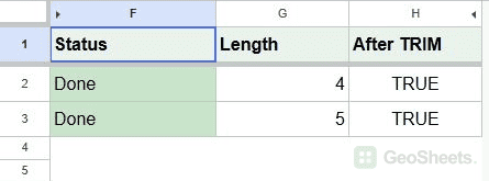
Two status labels can look identical but contain different characters. Imported text is especially worth checking when a rule matches one Done cell but skips another.

Suppose F2 contains Done, while F3 contains Done followed by a space. You can compare their lengths in spare cells:

=LEN(F2)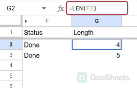

That returns 4 for the clean label. The same formula referencing F3 returns 5, revealing the extra character.

If you want your formatting rule to tolerate ordinary leading and trailing spaces, use this custom formula for F2:F3:

=TRIM(F2)="Done"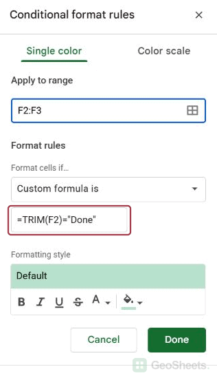

Both labels now qualify. TRIM cleans the text for the comparison; it doesn’t rewrite the contents of F2 or F3.

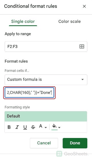
Text copied from websites can contain nonbreaking spaces, which TRIM doesn’t remove. If that’s the character causing the mismatch, replace it before trimming:

=TRIM(SUBSTITUTE(F2,CHAR(160)," "))="Done"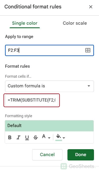

Don’t add increasingly complicated cleanup without checking the data first. A different status spelling needs a different correction from a hidden space.

Check whether numbers and dates are stored as text

A value that looks like 125 isn’t necessarily stored as a number. Similarly, a date imported from a CSV may still be text, even if it looks like your other dates.

Let’s say the questionable value is in D2. In a spare cell, enter:

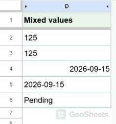
=ISNUMBER(D2)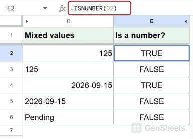

A genuine number returns TRUE. A numeric string returns FALSE. Dates recognized by Sheets are stored as numbers, so this also helps distinguish recognized dates from text.

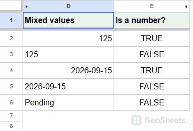
If D2 is the text 125, try this in a separate cell:

=VALUE(D2)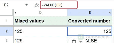

The result is the number 125. Check the converted result before replacing your original data, particularly when imported punctuation or date conventions differ from your spreadsheet’s locale.

For a rule that intentionally accepts numeric text, you could apply this to D2:D10:

=IFERROR(AND(D2<>"",VALUE(D2)>100),FALSE)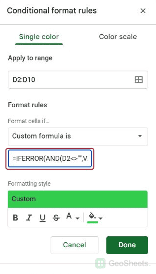

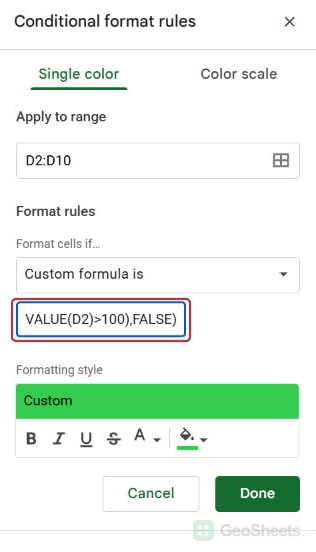
Both numeric 125 and text 125 qualify. Blank cells and unconvertible text such as Pending do not. The rule changes the comparison, not the stored values.

For text dates, try =DATEVALUE(D2) in a spare cell and format that result as a date. Confirm the day and month before relying on it.

Changing a cell’s display to Date alone isn’t a dependable way to parse ambiguous imported text. Once the underlying date is correct, your date-based formatting can compare it meaningfully.

Reorder overlapping rules when you see the wrong color

Sometimes the condition is correct, but another rule is supplying the color you see. Let’s return to the task table with Done and Open statuses in B2:B5.

Imagine you have a yellow rule for every nonempty status and a green rule for Done. A completed task satisfies both.

If the yellow rule is first, it takes priority. The green rule can be correct and still never supply the visible color for those cells.

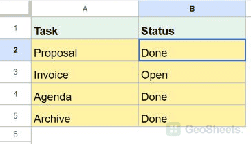
Here are the steps to give completed tasks priority:

1. Select a cell in the affected range and open Format > Conditional formatting.

   

2. Find the green rule using =$B2="Done".

   

3. Drag it above the yellow rule using =$B2<>"".

   

4. Check a Done row and an Open row.

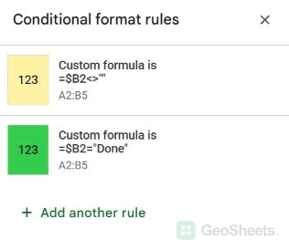
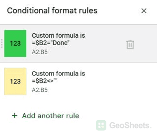
The Done rows should now be green, while the Open row remains yellow. Google specifies that the first matching rule defines the format.

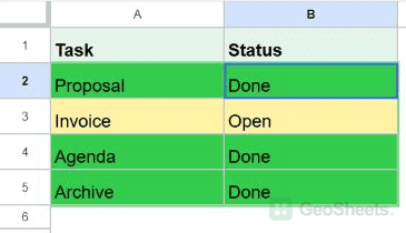
Another option is to make the yellow rule apply only to Open. Then the two conditions no longer overlap, making their order less important.

If a color appeared after pasting data, inspect the rule list too. Copying cells with conditional formatting can bring their rules with them.

Exclude cells that look blank

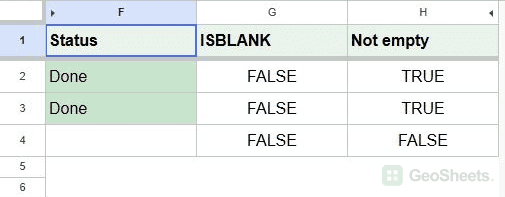
A cell containing a formula such as ="" looks blank, but it isn’t an empty cell. That difference matters if your condition uses ISBLANK.

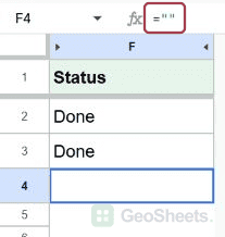
Suppose F4 contains that formula. =ISBLANK(F4) returns FALSE, because F4 contains a formula even though its displayed result is empty.

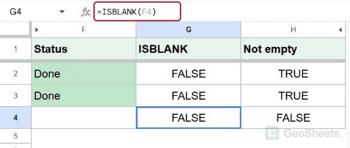
If you want to exclude both empty cells and empty-string results, include a comparison to an empty string in your rule:

=F2<>""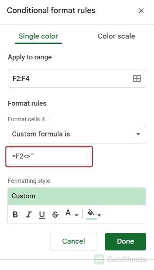

Applied to F2:F4, this leaves the empty-string result unhighlighted. A cell containing a space still counts as text, so investigate spaces separately if needed.

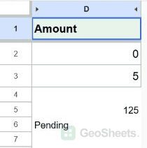
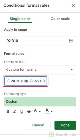
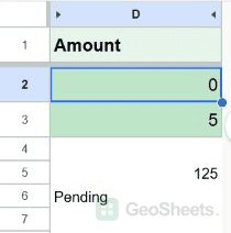
For numeric rules, a numeric check is often more useful. To highlight numbers below 10 in D2:D10 without coloring blanks, use:

=AND(ISNUMBER(D2),D2<10)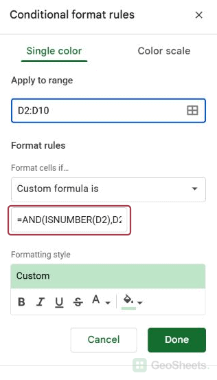

A genuine zero still qualifies. If zero means missing data in your sheet, add a separate D2<>0 condition rather than treating zero and blank as interchangeable.

Use INDIRECT when the rule refers to another tab

A formula can work in an ordinary cell and still be rejected in the conditional-formatting sidebar. A direct reference to another tab is one situation where this happens.

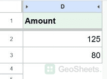
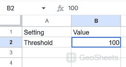
Suppose your amounts are in D2:D10, and a tab named Limits stores the threshold 100 in B2. You want to highlight numeric amounts above that threshold.

Instead of entering a direct Limits reference in the rule, select D2:D10 and use:

=AND(ISNUMBER(D2),D2>INDIRECT("'Limits'!$B$2"))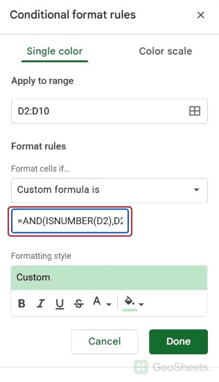

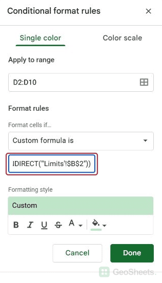
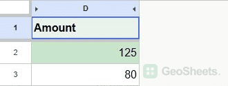
A numeric amount of 125 qualifies; 80 does not. INDIRECT turns the text address into the reference the rule needs.

The single quotes around Limits also work with tab names containing spaces, such as 'Project Limits'!$B$2. Keep the actual tab name spelled exactly as it appears in your workbook.

If you rename that tab, update the text inside INDIRECT too. For more examples, see conditional formatting across sheets.

Extend the rule when new rows are skipped

If your original records format correctly but newly added records do not, check where the rule stops. A rule ending at row 5 cannot format a new task in row 6.

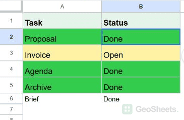
For the task table, changing Apply to range from A2:B5 to A2:B6 includes the new record. Keep the formula =$B2="Done" because the first data row hasn’t changed.

If you regularly append tasks, you can use an open-ended range such as A2:B. It covers the available rows below the heading, including new entries.

For rules that compare against a list, check the comparison range too. Expanding the colored area doesn’t automatically expand a fixed range inside MAX, MIN, or COUNTIF.

After changing the range, check one matching row, one nonmatching row, and the newest record. That shows whether the rule reaches the new data and still evaluates each row correctly.

Other Google Sheets articles you may also like

• Highlight an Entire Row Based on Another Cell
• Highlight Cells Containing Specific Text
• Fill Color Options for One-Off Highlighting