Highlight Cells Containing Specific Text in Google Sheets

When you’re looking through a task list or customer notes, you may want certain words to stand out. Highlighting entries containing “urgent,” for example, makes them easier to spot as you scroll.

Google Sheets can do this automatically with conditional formatting. You can look for a fixed word, use a search term from another cell, or match several words at once.

In this tutorial, I’ll show you those approaches, along with exact matches, case-sensitive searches, and whole-word matches when you don’t want to highlight part of a longer word.

Highlight cells with the Text contains rule

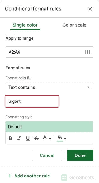
Let’s start with the simplest option. Below, I have a short task list in A2:A6, and I want any task containing urgent to stand out.

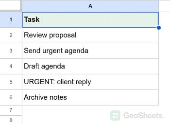
You don’t need a formula for this. Sheets has a built-in Text contains condition that searches inside each selected cell.

Here are the steps to highlight tasks containing urgent:

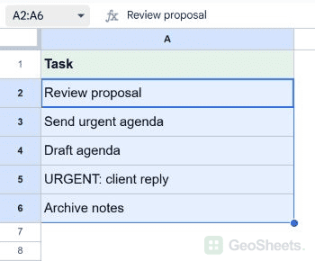
1. Select A2:A6.

   

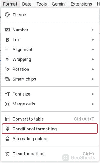
2. Click Format > Conditional formatting.

   

3. Check that Apply to range shows A2:A6.
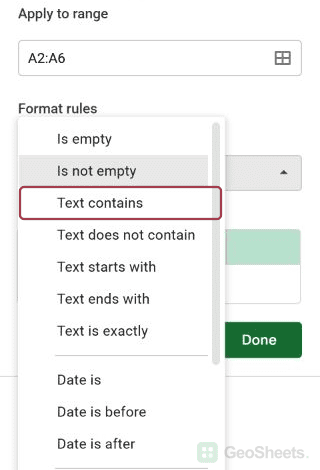
4. Under Format cells if, select Text contains.

   

5. Enter urgent in the value field, without quotation marks.

   

6. Choose a fill color under Formatting style and click Done.

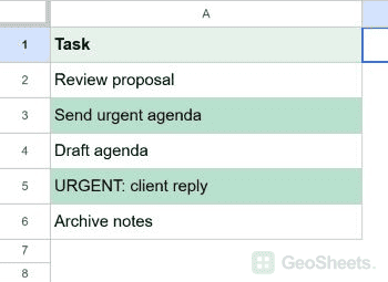
Cells A3 and A5 are highlighted. The word can appear anywhere in the cell, and capitalization doesn’t matter for this rule.

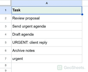
The highlighting updates when you edit your tasks. For example, adding urgent to Archive notes makes that cell match too.

However, Text contains also matches urgent inside nonurgent. If you need a separate word rather than any matching sequence of letters, use the whole-word method later in this tutorial.

Match literal question marks and asterisks

There are two special characters to know about in Text contains. An asterisk matches any sequence of characters, while a question mark matches one character.

If you’re looking for a literal question mark, add a tilde before it. For example, urgent~? searches for urgent? rather than treating the question mark as a wildcard.

Similarly, ~* searches for an actual asterisk. Google describes these patterns in its conditional formatting documentation.

Highlight only cells whose entire text matches

Sometimes you’re working with short labels, such as Urgent, Open, and Closed. You may want the Urgent label highlighted without also highlighting Send urgent agenda.

That’s a whole-cell match. It differs from both a partial-text search and a whole-word search inside a sentence.

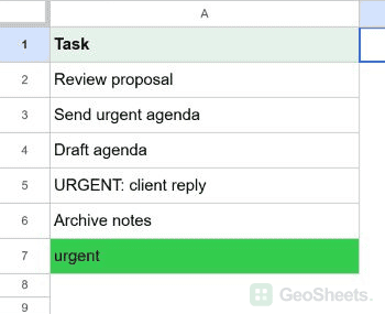
To see the difference, add urgent in A7 beneath the task list, then use these steps:

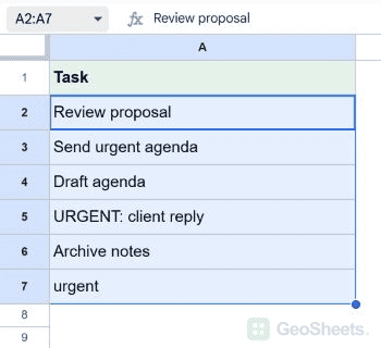
1. Select A2:A7 and open Format > Conditional formatting.

   

   

2. Edit the existing text rule, or remove it before adding this replacement.
3. Choose Text is exactly under Format cells if.

   

4. Enter urgent, choose a fill, and click Done.

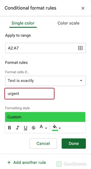
Now A7 matches, while the longer task descriptions do not. Removing the earlier Text contains rule lets you see the effect of this more specific condition.

Whole-cell matching and case-sensitive matching are different requirements. If capitalization is part of your requirement too, use =EXACT(A2,"urgent") as a custom formula for this range.

Use another cell as your search term

If you regularly search for different words, editing the sidebar each time gets inconvenient. Instead, you can type your search term into a cell and let the rule read it from there.

For this example, the tasks are in A2:A6. I’ll put the label Search term in B1 and urgent in B2.

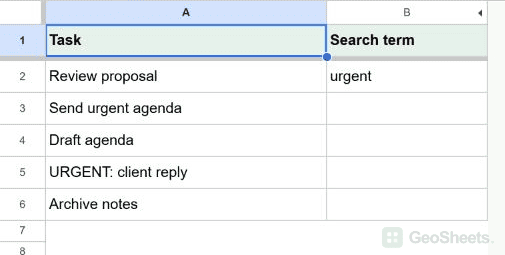
Here are the steps to connect the highlighting to B2:

1. Enter urgent in B2.
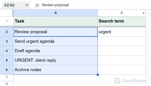
2. Select A2:A6, then open Format > Conditional formatting.

   

   

3. Replace any earlier rule for this example, so its color doesn’t hide the new rule.
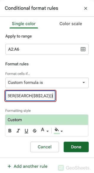
4. Choose Custom formula is and enter the formula below.
5. Select a fill color and click Done.

=AND($B$2<>"",ISNUMBER(SEARCH($B$2,A2)))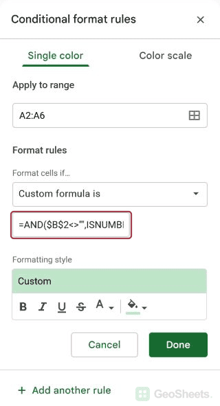

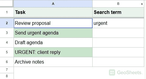
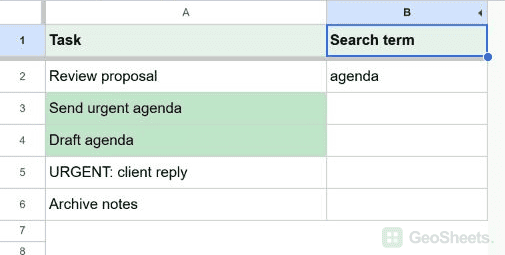
With urgent in B2, A3 and A5 are highlighted. Now replace urgent with agenda. The highlighting moves to A3 and A4, without any changes in the sidebar.

SEARCH($B$2,A2) looks for your search term inside each task. When it finds a match, it returns a position, and ISNUMBER turns that into a TRUE result for the formatting rule.

The $B$2 reference stays fixed on your search cell. The A2 reference moves down the task list, letting each task receive its own result.

The extra $B$2<>"" check matters too. If you clear B2, the rule stops highlighting cells instead of searching for an empty string.

If your list starts in C5 instead, select C5:C20 and change A2 to C5. Keep B2 fixed if that’s still where you type the search term.

Our absolute reference guide explains how the dollar signs control which parts of a reference can change.

Highlight text only when the capitalization matches

Suppose lowercase urgent and uppercase URGENT mean different things in your list. SEARCH ignores capitalization, so it won’t distinguish between them.

Let’s use the tasks in A2:A6 and lowercase urgent in B2 again. This time, I want Send urgent agenda highlighted, but not URGENT: client reply.

Here are the steps to make that search case-sensitive:

1. Select A2:A6 and open Format > Conditional formatting.

   

   

2. Edit your custom rule, or create one if you don’t already have it.
3. Choose Custom formula is and enter the formula below.
4. Choose a fill color and click Done.

=AND($B$2<>"",ISNUMBER(FIND($B$2,A2)))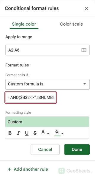

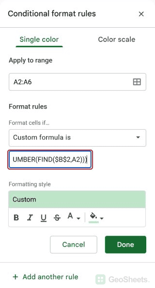
Only A3 matches. FIND looks for the same text as SEARCH, but capitalization must match. The empty-search check still switches the rule off when B2 is cleared.

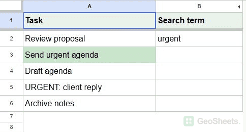
This still searches within a longer sentence. If you want the entire cell to equal lowercase urgent, use the EXACT formula in the whole-cell section instead.

Highlight cells containing either of two words

You may want to review both urgent tasks and tasks mentioning an invoice. One rule can highlight either group in the same color.

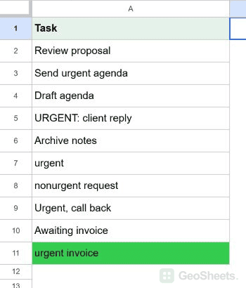
For this example, let’s extend the task list to A11 with the following entries:

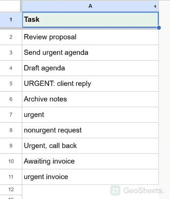
Here are the steps to highlight either word:

1. Select A2:A11 and open Format > Conditional formatting.

   

   

2. Create a Custom formula is rule.
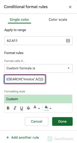
3. Enter the formula below, choose a fill color, and click Done.

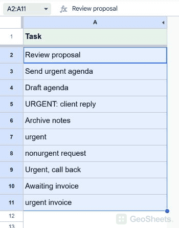
=OR(ISNUMBER(SEARCH("urgent",A2)),ISNUMBER(SEARCH("invoice",A2)))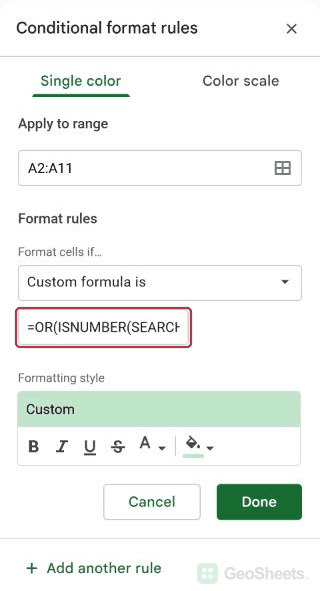

The highlighted cells are A3, A5, A7, A8, A9, A10, and A11. OR means either search may succeed; a cell containing both words qualifies too.

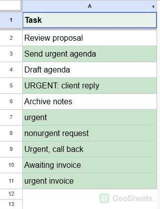
A8 is included because nonurgent contains the letters urgent. These are substring searches, just like the earlier Text contains example.

If you want different colors for urgent and invoice, create two separate rules instead. A task containing both terms will need a priority: drag the preferred rule above the other one.

Require both words in the same cell

Perhaps you only want urgent invoices. With the same task list in A2:A11, replace OR with AND:

=AND(ISNUMBER(SEARCH("urgent",A2)),ISNUMBER(SEARCH("invoice",A2)))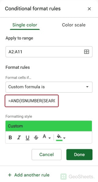

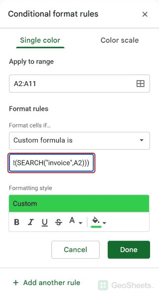
Now only A11 matches. Both words must be present, though they don’t have to appear in a particular order or next to one another.

Highlight a whole word without matching longer words

If nonurgent keeps getting highlighted when you search for urgent, a whole-word match can help. Let’s keep the extended task list in A2:A11 and exclude that longer word.

We’ll use REGEXMATCH, which lets you describe a text pattern. You only need a small pattern here: the word urgent with a boundary on either side.

Remove the earlier text-search rules from A2:A11 before trying this method. Otherwise, their substring matches can keep nonurgent highlighted even though the whole-word rule excludes it.

Here are the steps to apply the whole-word rule:

1. Select A2:A11 and open Format > Conditional formatting.

   

   

2. Create or edit a Custom formula is rule.
3. Enter the formula below, choose a fill, and click Done.

=IFERROR(REGEXMATCH(A2,"(?i)\burgent\b"),FALSE)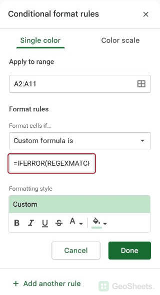

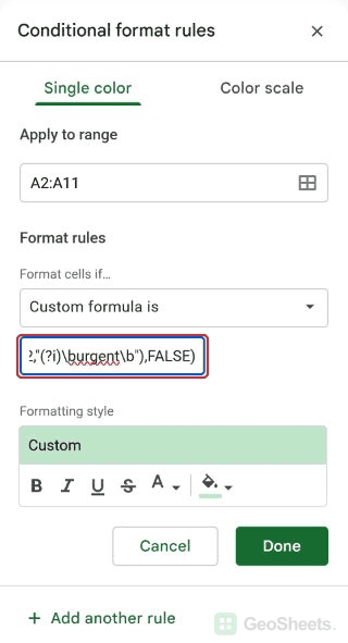
This highlights A3, A5, A7, A9, and A11. It includes Urgent followed by a comma and URGENT followed by a colon, but leaves nonurgent request unhighlighted.

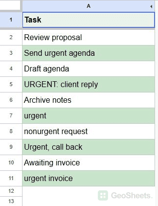
The (?i) makes the match case-insensitive. Each \b marks a word boundary. IFERROR returns FALSE if the cell contains something the text function can’t evaluate, such as a number.

You can replace urgent with another plain English word. A word containing punctuation, such as C++, needs a different pattern because punctuation can have a special meaning in regular expressions.

These word boundaries follow RE2’s definition, which uses ASCII letters, digits, and underscores. They aren’t a reliable language-aware boundary for every accented or non-Latin word.

Google’s REGEXMATCH reference explains its use of RE2. For ordinary English labels such as urgent or invoice, the pattern above keeps the distinction clear.

Highlight the entire row based on text in one column

Once you’ve found the matching tasks, you may want their other details highlighted too. For example, your task descriptions could be in A2:A11 with an owner and deadline in columns B and C.

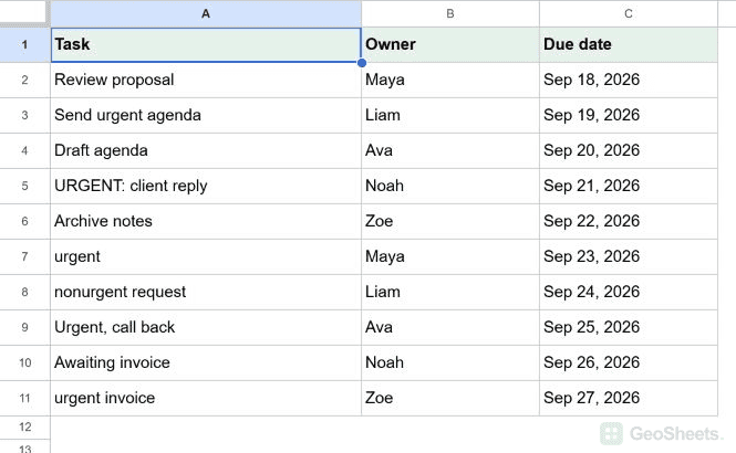
For that layout, select A2:C11 and create a custom conditional-formatting rule with:

1. Select A2:C11 so the task, owner, and due-date cells can all be colored.

   

2. Choose Format > Conditional formatting.

   

3. Choose Custom formula is, enter the formula below, and choose a fill.
4. Click Done.

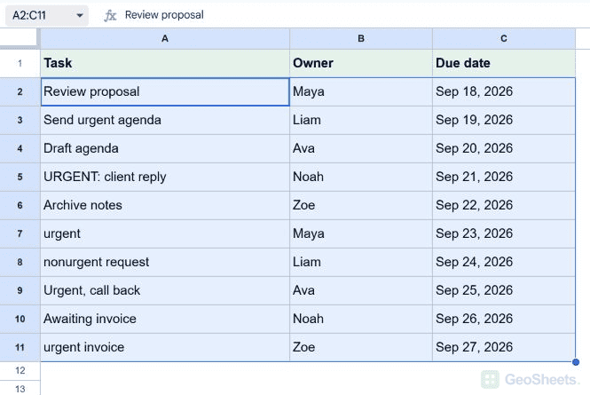
=ISNUMBER(SEARCH("urgent",$A2))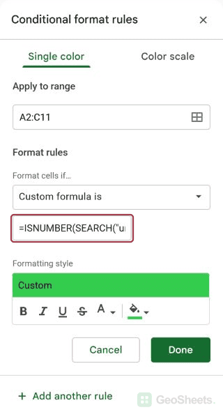

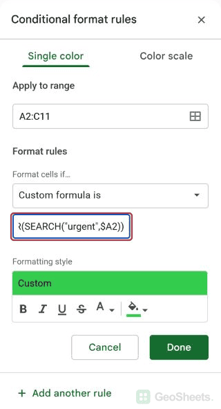
Each matching task colors the cells across A:C in its row. The $A2 reference keeps the condition checking the task column as the formatting extends to the other columns.

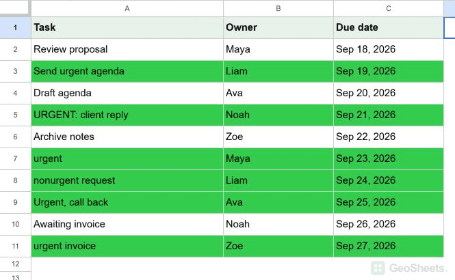
This example uses a fixed search term, leaving columns B and C available for your data. See our row-highlighting tutorial for other conditions you can use.

Other Google Sheets articles you may also like

• How to Count Cells with Text in Google Sheets
• Use Multiple Conditions in Conditional Formatting
• Fix Conditional Formatting That Is Not Working