Conditional Formatting With Multiple Conditions in Google Sheets

When you’re reviewing a task list, highlighting every high-priority task might not be enough. You may only want the ones still in progress, or anything that’s overdue and hasn’t been completed.

In Google Sheets, you can combine those requirements in a conditional formatting formula. That lets you highlight exactly the cells or rows you want without checking each record yourself.

In this tutorial, I’ll show you how to combine conditions with AND and OR, mix them in one formula, and use separate colors when different conditions need different highlights.

Highlight rows when both conditions are true

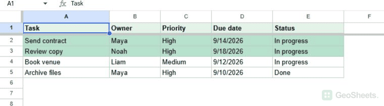
Below, I have a task list in A1:E5. I want to highlight tasks that have High priority and are still In progress.

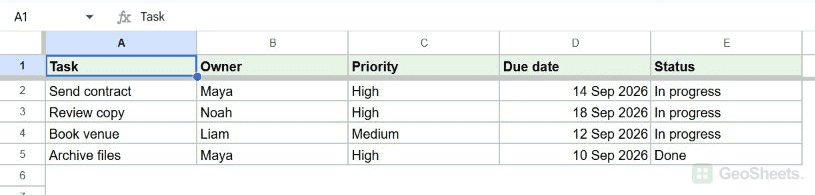
Let’s apply a green fill to the rows that meet both requirements.

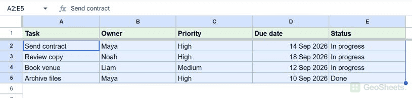
1. Select A2:E5, leaving out the headings.

   

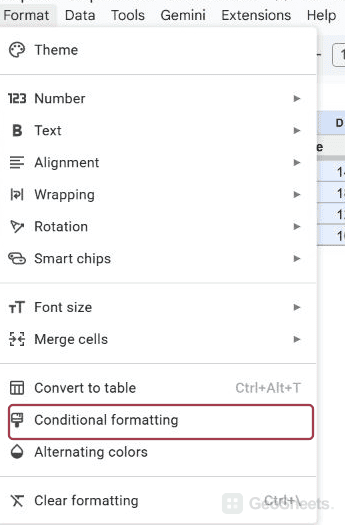
2. Go to Format > Conditional formatting.

   

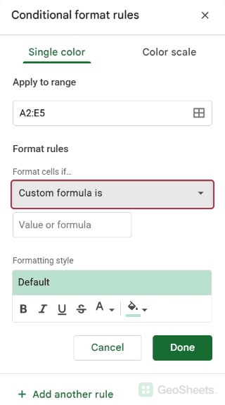
3. Under Format cells if, choose Custom formula is.

   

4. Enter the formula below.
5. Choose a green fill under Formatting style, then click Done.

=AND($C2="High",$E2="In progress")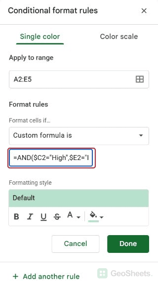

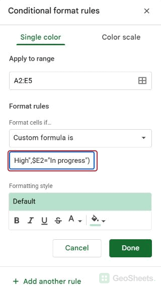
Send contract and Review copy are highlighted. Book venue doesn’t qualify because its priority is Medium. Archive files doesn’t qualify because it’s already Done.

The AND function checks both comparisons. It returns TRUE only when column C contains High and column E contains In progress in the same row.

If your labels are different, replace the words inside quotation marks. For example, use “Open” if that’s the status your team uses for unfinished work.

Why the dollar signs matter

We’re formatting five columns, but every cell in a row must check that row’s Priority and Status. The dollar signs keep those checks in columns C and E.

Reference	What changes as Sheets checks other cells	Use here?
$C2	The row changes; column C stays fixed	Yes, check each task’s priority
$C$2	Nothing changes	No, every task would check C2
C2	Both column and row can change	No, checks would shift across the highlighted row

The first row number also needs to match your selected range. For A2:E5, we start with row 2. If your data begins at row 10, use $C10 and $E10 instead.

To highlight only the task names, change Apply to range to A2:A5. The formula stays the same because the conditions still live in C and E.

Highlight rows when either condition is true

Now let’s look at a different requirement: highlight anything that’s High priority or Blocked. This time, satisfying either requirement should be enough.

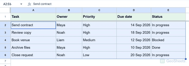
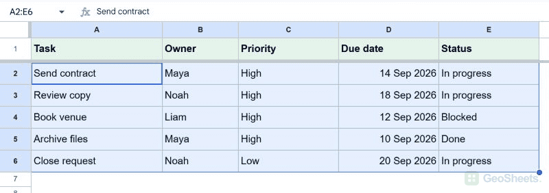
For this example, I have the same columns in A:E, but Book venue is Blocked. I’ve also added Close request in row 6, with Low priority and In progress status.

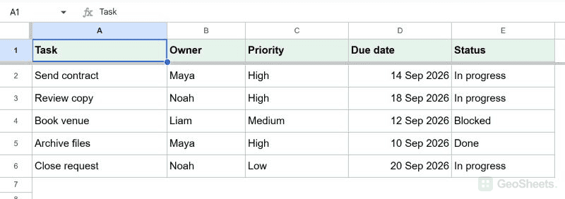
Here are the steps to highlight either type of task.

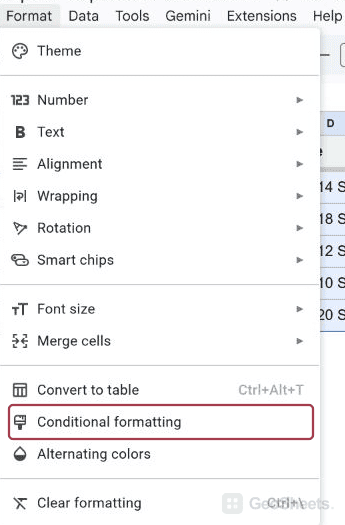
1. Select A2:E6 and open Format > Conditional formatting.

   

   

2. Choose Custom formula is.
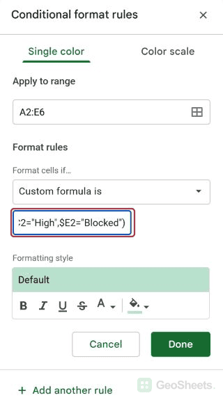
3. Enter the OR formula below.
4. Choose a fill color and click Done.

=OR($C2="High",$E2="Blocked")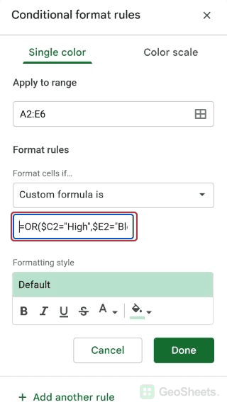

Send contract, Review copy, Book venue, and Archive files all qualify. Close request doesn’t, because it’s neither High priority nor Blocked.

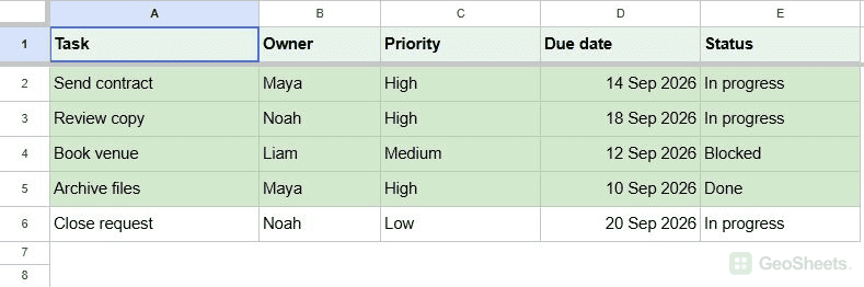
Notice that Archive files still qualifies even though it’s Done. OR doesn’t know that completed work should be excluded unless we explicitly add that requirement.

If you’re comparing this with the previous example on the same sheet, remove the old rule first. Otherwise, two rules may be coloring the same rows.

Match either of two values in the same column

OR can also check several possible values in one column. For example, you might want to highlight both High and Medium priorities while leaving Low tasks alone.

With Priority in column C and the applied range set to A2:E6, choose Custom formula is and enter this formula:

=OR($C2="High",$C2="Medium")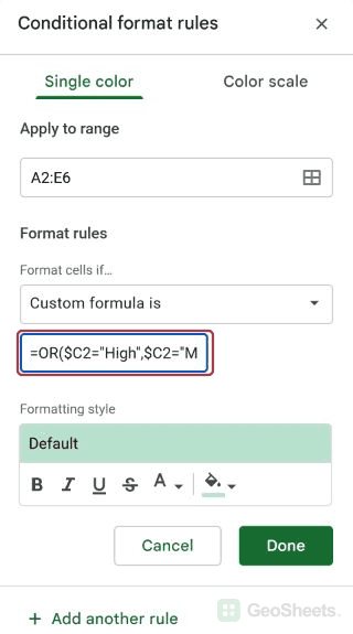

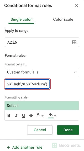
Both comparisons check column C. In this list, rows 2 through 5 qualify, while the Low-priority task in row 6 stays unchanged.

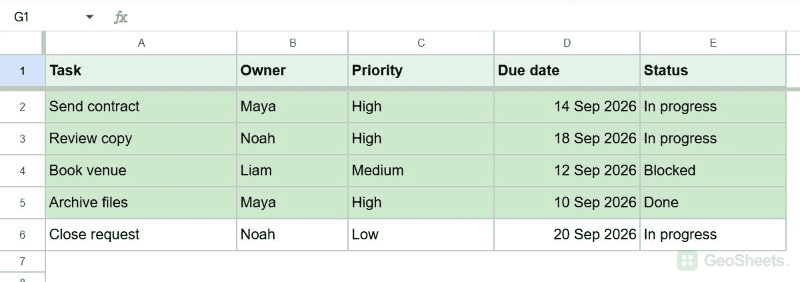
Don’t use AND for this requirement. One cell can’t be exactly “High” and exactly “Medium” at the same time, so neither value would qualify.

Combine AND and OR to exclude completed tasks

Suppose you want to highlight High-priority or Blocked tasks, but only while they’re unfinished. We can put OR inside AND to express that combination.

For the task list in A1:E6, Priority is in C and Status is in E. We’ll keep the entire row as our formatting range.

Let’s replace the simpler OR rule with this more selective one.

1. Select A2:E6 and open Format > Conditional formatting.

   

   

2. Click the existing rule to edit it, or add a rule and choose Custom formula is.
3. Enter the formula below, choose a fill, and click Done.

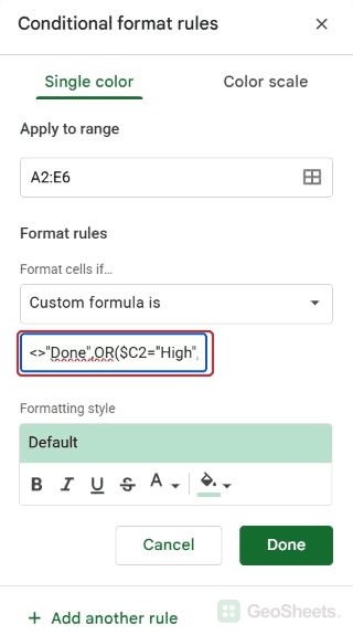
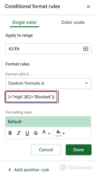
=AND($E2<>"Done",OR($C2="High",$E2="Blocked"))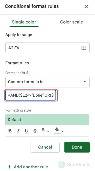

Now Send contract, Review copy, and Book venue qualify. Archive files drops out because its Done status makes the first condition false.

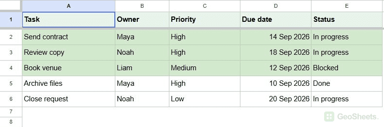
Read the formula from the outside: the task must not be Done, and the group inside OR must also be true. Within that group, either High priority or Blocked status is enough.

The <> operator means “not equal to.” If you use Completed instead of Done, replace that label in the formula.

Combine text conditions with a numeric threshold

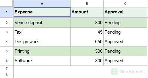
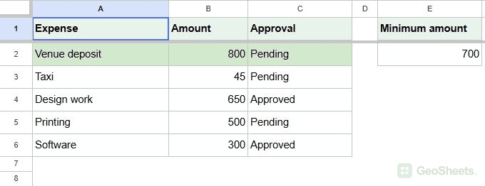
You aren’t limited to status labels. Below, I have an expense list in A1:C6, and I want to highlight Pending expenses of at least 500.

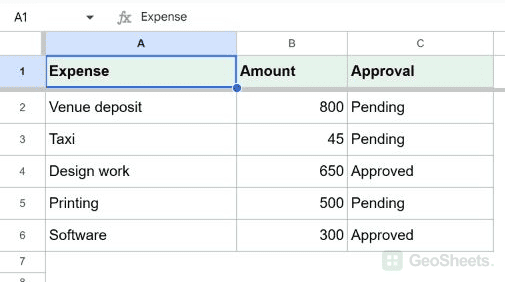
Here’s how to combine the amount and approval checks.

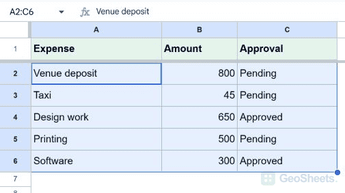
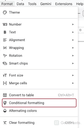
1. Select A2:C6 and open Format > Conditional formatting.

   

   

2. Choose Custom formula is and enter the formula below.
3. Choose a fill color, then click Done.

=AND(ISNUMBER($B2),$B2>=500,$C2="Pending")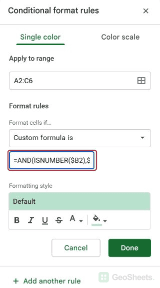

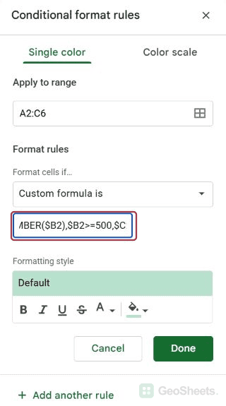
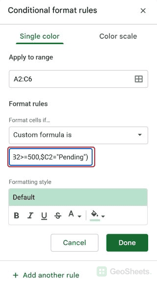
Venue deposit and Printing qualify. Printing is included because >=500 means 500 or more, rather than strictly more than 500.

ISNUMBER requires an actual number in B. A blank cell or a number stored as text won’t qualify, even if it looks like an amount on screen.

If the minimum changes regularly, put 500 in E2 and use this version instead:

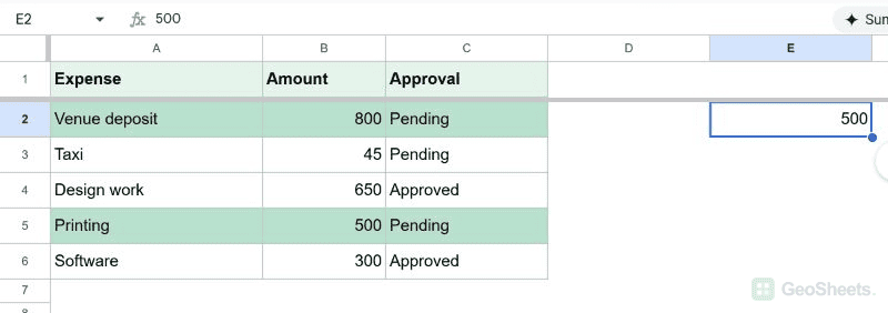
=AND(ISNUMBER($B2),$B2>=$E$2,$C2="Pending")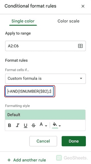

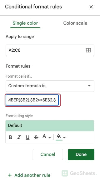
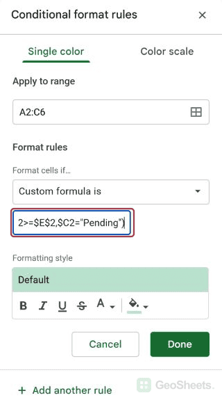
Here, $E$2 deliberately locks both the column and row. Every expense compares against the same threshold. Changing E2 to 700 leaves only Venue deposit highlighted.

Combine a due date with priority and status

For a task tracker, you might want to highlight only overdue, High-priority work that isn’t Done. That combines three business requirements in one rule.

In this example, the list occupies A1:E5: Task, Owner, Priority, Due date, and Status. Enter real dates in D, with some before today and some after it.

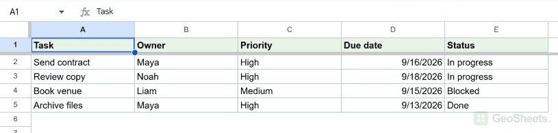
To highlight the qualifying tasks, apply a custom formula to A2:E5:

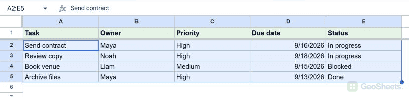
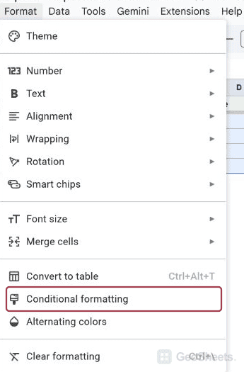
1. Select A2:E5, leaving out the headings.

   

2. Choose Format > Conditional formatting.

   

3. Under Format cells if, choose Custom formula is and enter the formula below.
4. Choose a fill color and click Done.

=AND(ISNUMBER($D2),$D2<TODAY(),$C2="High",$E2<>"Done")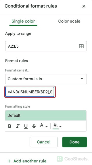

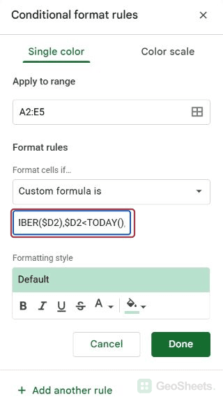
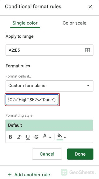
A High-priority task due yesterday qualifies if it’s unfinished. A task due today, a future task, or a completed task doesn’t. A blank or text date also stays unhighlighted.

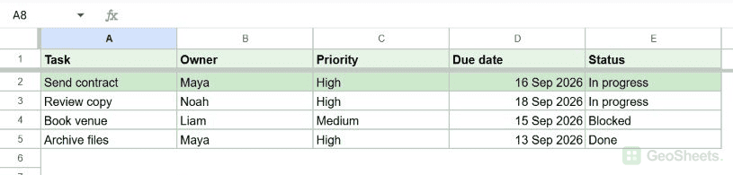
ISNUMBER checks that the date is numeric, which is how Sheets stores real dates. TODAY supplies the current date, and the less-than comparison finds dates before it.

If you don’t need the priority requirement, see the fuller guide to highlighting overdue dates, including completion checkboxes and aging thresholds.

Use separate rules for different colors

Combining conditions is useful when every matching row should look the same. But you may want Blocked tasks in red and other High-priority tasks in yellow.

For a task list in A1:E6, with Priority in C and Status in E, create two custom rules applying to A2:E6.

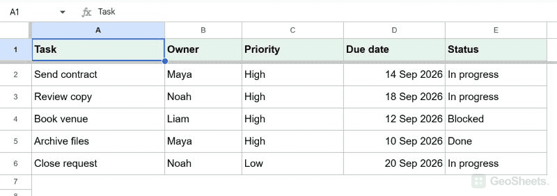
Let’s add the red rule first.

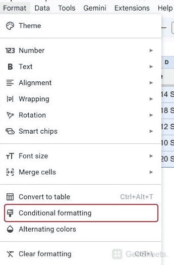
1. Open Format > Conditional formatting for A2:E6.

   

   

2. Choose Custom formula is and enter the first formula below.
3. Choose a red fill and click Done.
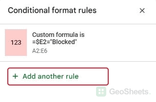
4. Click Add another rule, use the same range, and enter the second formula.

   

5. Choose a yellow fill and click Done.

The red rule is:

=$E2="Blocked"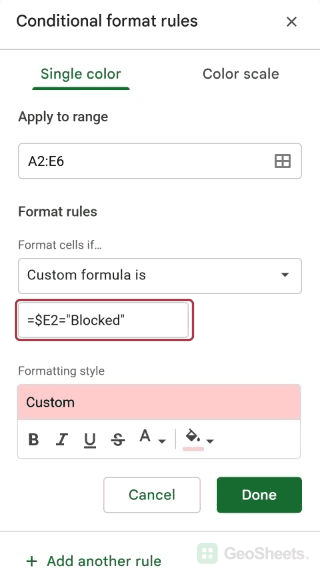

The yellow rule is:

=$C2="High"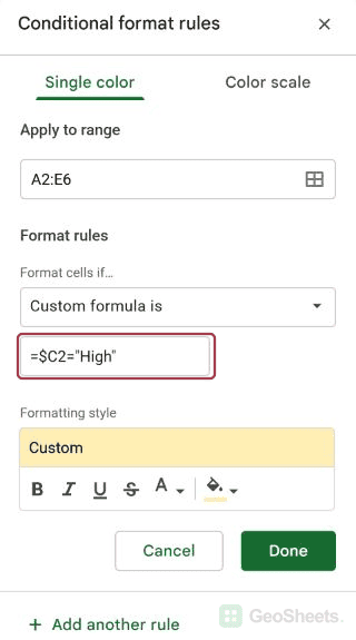

A task that’s both High priority and Blocked matches both rules. Drag the Blocked rule above the High rule so that the red warning takes precedence.

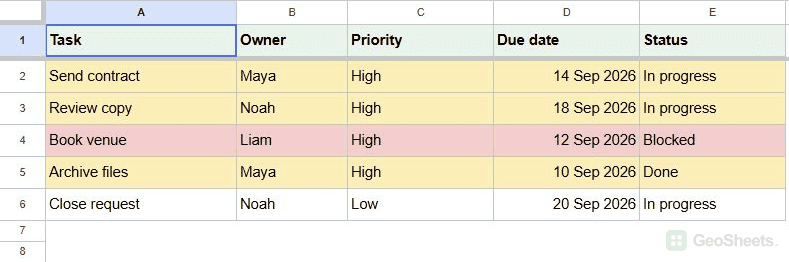
Google documents that the first matching rule determines the format. Reversing these rules would give that overlapping task the yellow fill instead.

You can also prevent overlap by making the yellow rule more specific:

=AND($C2="High",$E2<>"Blocked")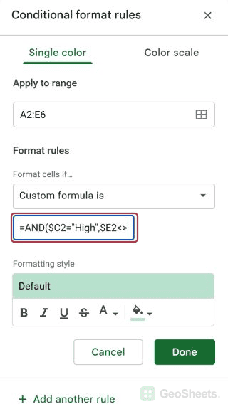

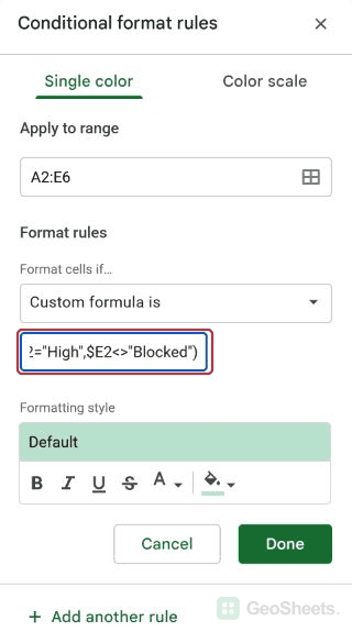
Now the yellow rule excludes Blocked tasks entirely. This is useful when you want each color to represent a distinct category, regardless of how the rules are ordered.

Choose AND, OR, or separate formatting rules

When you create another rule, decide whether every requirement must match or one is enough. This comparison summarizes the methods you’ve just tried.

What you want	Use	Example
Every condition must match	AND	High priority and still in progress
At least one condition must match	OR	High priority or blocked
One requirement plus a choice of others	AND with OR inside it	Not completed, and either high priority or blocked
Different highlights for different situations	Separate rules	Blocked tasks red; other high-priority tasks yellow

One formula produces one TRUE or FALSE result for each cell being evaluated. A TRUE result applies the style you chose. You don’t need to wrap the formula in IF.

Other Google Sheets articles you may also like

• Conditional Formatting in Google Sheets
• OR Function in Google Sheets
• Highlight an Entire Row Based on Another Cell