
When you’re managing tasks or tracking invoices in Google Sheets, it helps to see what’s overdue without checking every date against the calendar.
Conditional formatting can highlight those dates automatically. You can also exclude completed work, color the entire row, or flag only items that are several days late.
In this tutorial, I’ll show you how to set up each of those options, starting with a simple list of dates and then adding the conditions a task tracker needs.
Highlight past dates with a built-in rule
If you only have a list of dates, you don’t need a custom formula. Google Sheets has a built-in condition for dates before today.
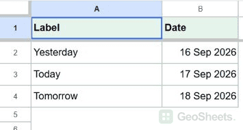
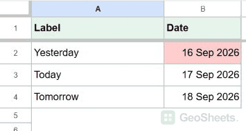
Below, I have three deadlines in B2:B4: yesterday, today, and tomorrow. I want yesterday’s date to stand out while leaving the other two unchanged.
You can use your own dates, or enter =TODAY()-1, =TODAY(), and =TODAY()+1 in those cells to follow along.
Here are the steps to highlight the dates that have passed.
- Select
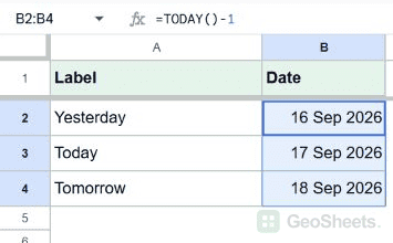
B2:B4.
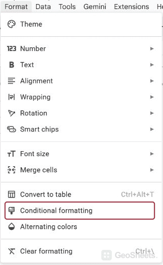
- Go to Format > Conditional formatting.

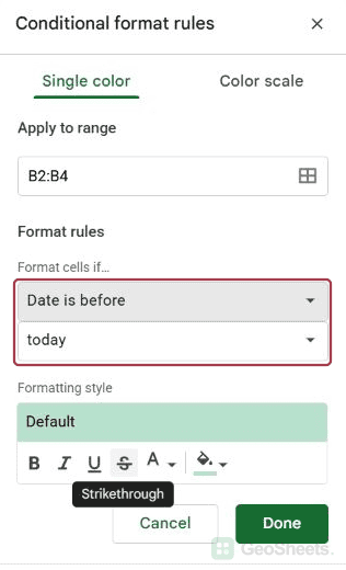
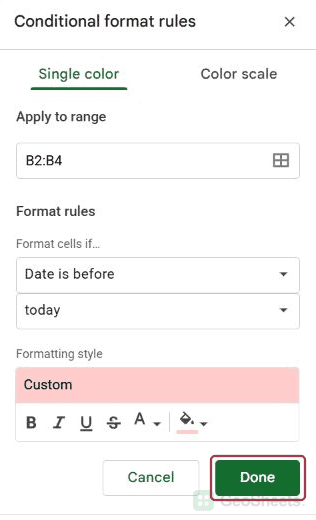
- Under Format cells if, choose Date is before.

- Choose today as the comparison date.
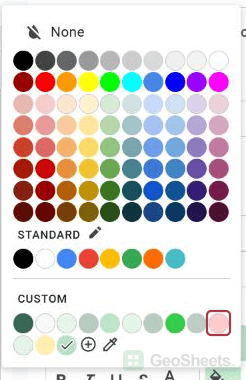
- Choose a red fill under Formatting style, then click Done.

Yesterday’s date is highlighted. Today and tomorrow aren’t, because “before today” means the date has already passed.
This rule only checks the dates you selected. It doesn’t know whether a task has been completed or an invoice has been paid. Let’s add that distinction next.
Highlight overdue tasks but exclude completed work
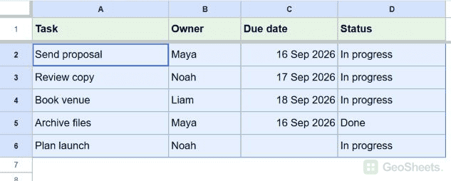
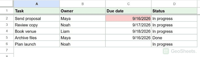
Below, I have a task tracker in A1:D6. The due date is in column C, and column D tells me whether the task is Done.
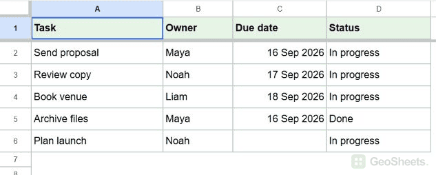
These screenshots use September 17, 2026 as today. In your sheet, use real dates or the TODAY formulas from the previous section, and leave C6 empty.
I want only Send proposal highlighted. Its deadline has passed, it isn’t Done, and it has a real due date.
Let’s create a rule that checks all three requirements.
- Select
A2:D6so the whole task row can be highlighted.
- Choose Format > Conditional formatting.
- Under Format cells if, select Custom formula is.

- Enter the formula below.
- Choose a red fill, then click Done.
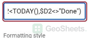
=AND(ISNUMBER($C2),$C2<TODAY(),$D2<>"Done")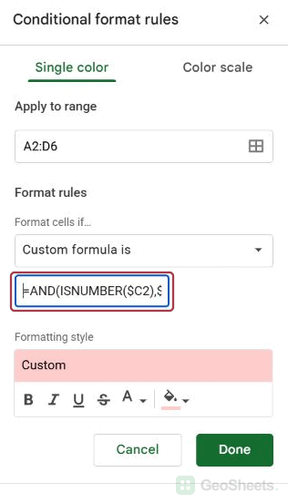
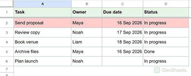
Send proposal receives the highlight. Review copy and Book venue aren’t overdue, Archive files is finished, and Plan launch has no date to compare.
Here’s what each part checks:
ISNUMBER($C2)requires a numeric date value, excluding empty cells and text.$C2<TODAY()checks whether the due date is earlier than today.$D2<>"Done"excludes completed tasks. The<>symbol means “not equal to.”
AND requires all three checks to pass. You can change Done to Paid, Complete, or whichever label identifies finished items in your list.
If your due-date column already contains only real dates or blanks, this simpler version also excludes empty cells:
=AND($C2<>"",$C2<TODAY(),$D2<>"Done")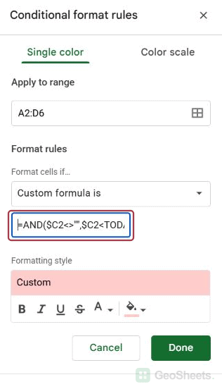
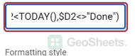
I prefer the ISNUMBER version when dates arrive from copied or imported data. It makes the requirement clearer: the due date must be stored as a number, not merely look like a date.
Highlight only the date instead of the whole row
The formula decides which task qualifies. The Apply to range field decides which cells receive the color.
If you only want the date highlighted, open the rule and change its range from A2:D6 to C2:C6. Keep the same formula.
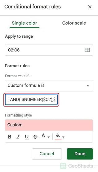
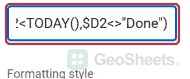
The dollar signs keep the checks in columns C and D. The row number stays flexible so row 3 checks C3 and D3, row 4 checks C4 and D4, and so on.
If your selected range begins at row 5, use $C5 and $D5 in the formula. Starting with the wrong row number makes the highlight appear beside the wrong task.
Include tasks due today
You may want today’s work included in the alert, even though its deadline hasn’t passed. We only need to change the date comparison.
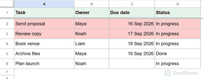
For a task list with due dates in C and status in D, apply this custom formula to A2:D6:
=AND(ISNUMBER($C2),$C2<=TODAY(),$D2<>"Done")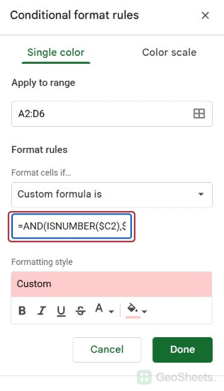
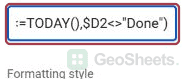
The extra equals sign includes dates equal to today. In the example above, both Send proposal and Review copy are highlighted.
This version assumes your cells contain dates without times. A timestamp for today at 3 p.m. is later than the date value returned by TODAY.

If your due dates include times and you want to include the whole of today, use a boundary before tomorrow instead:
=AND(ISNUMBER($C2),$C2<TODAY()+1,$D2<>"Done")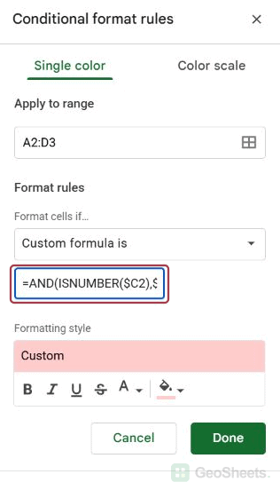
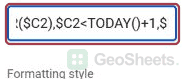
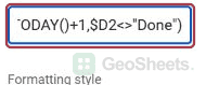
A deadline today at 3 p.m. now qualifies. A deadline exactly at midnight tomorrow doesn’t. This is a calendar-day alert, rather than a check of whether the current time has passed the deadline.

Exclude completed tasks using checkboxes
If your tracker uses a completion checkbox, you can check its value instead of looking for the word Done.
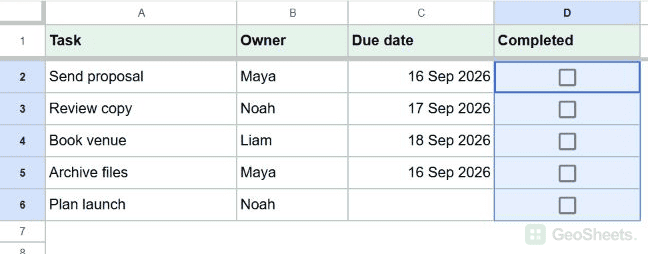
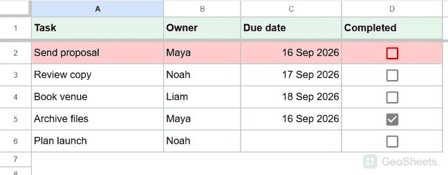
For this example, I have Task in A, Owner in B, Due date in C, and a Completed checkbox in D. Rows 2 through 6 contain the task list.
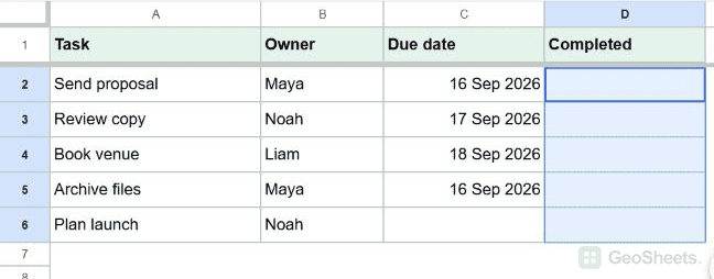
Here’s how to highlight overdue tasks whose completion boxes are still unchecked.
- If the checkboxes don’t exist yet, select
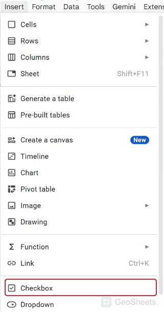
D2:D6and choose Insert > Checkbox.

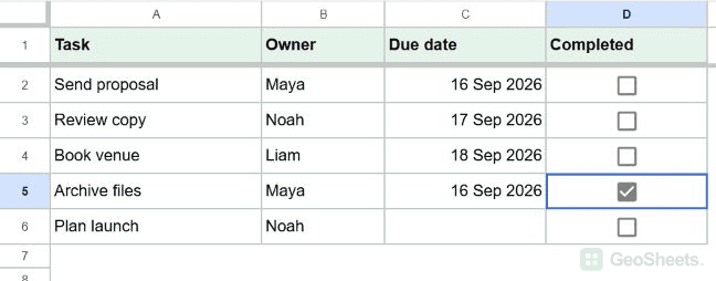
- Check the boxes for any finished tasks.
- Select
A2:D6, then choose Format > Conditional formatting. - Choose Custom formula is and enter the formula below.
- Choose a red fill and click Done.
=AND(ISNUMBER($C2),$C2<TODAY(),$D2=FALSE)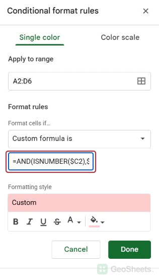
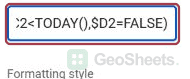
With default checkboxes, an unchecked box contains FALSE and a checked box contains TRUE. Checking the box removes that task’s overdue highlight; unchecking it makes the task eligible again.
This formula assumes default checkbox values. If you configured custom values such as Yes and No, replace $D2=FALSE with $D2="No" to match your unchecked value.
For completion styling itself, such as coloring finished rows green, see highlighting a row when a checkbox is checked.
Highlight tasks more than seven days overdue
Sometimes yesterday’s deadline and a month-old deadline shouldn’t receive the same attention. You can add an aging threshold to show tasks that are more than a certain number of days late.
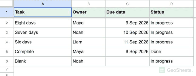
Below, I’m using due dates in C and status in D. Apply the following custom rule to your task rows, such as A2:D100:
=AND(ISNUMBER($C2),$C2<TODAY()-7,$D2<>"Done")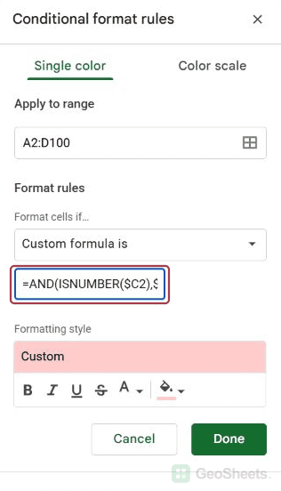
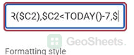
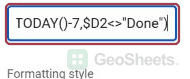
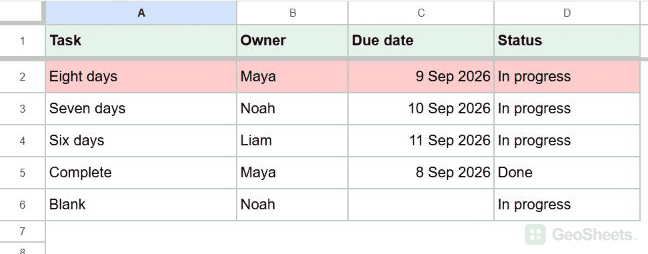
A task due eight days ago qualifies. A task due exactly seven days ago doesn’t, because the comparison is strictly less than the seven-day cutoff.
If you mean “seven or more days overdue,” include the cutoff date with this version:
=AND(ISNUMBER($C2),$C2<=TODAY()-7,$D2<>"Done")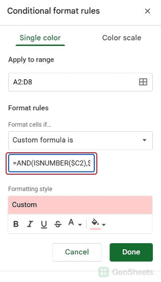
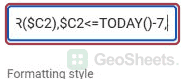
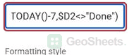
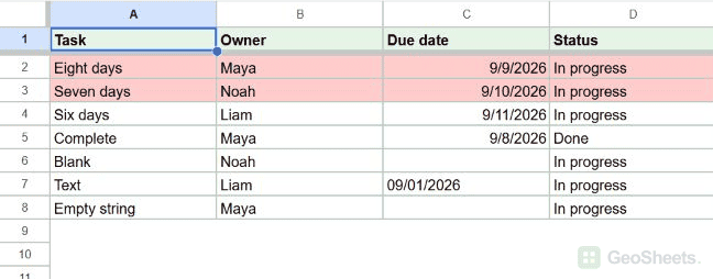
With the inclusive rule, Eight days and Seven days are highlighted. Six days stays unfilled, along with completed tasks, blank dates, and dates stored as text.
These formulas count calendar days, including weekends. A business-day escalation policy needs a different calculation, such as one based on NETWORKDAYS, along with your holiday list.
Change the threshold without editing the rule
If the cutoff changes, put the number of days in F2. For example, enter 7, then use this rule for tasks more than that many days overdue:
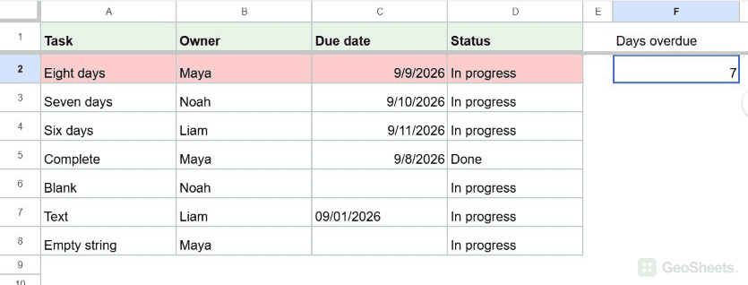
=AND(ISNUMBER($C2),$C2<TODAY()-$F$2,$D2<>"Done")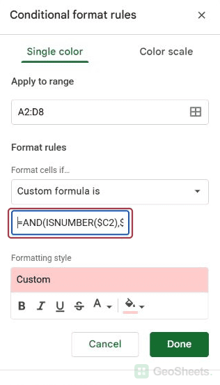
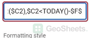
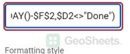
Changing F2 to 14 switches the alert to tasks more than two weeks late. Keep F2 numeric and nonnegative.
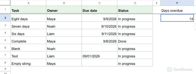
Both dollar signs in $F$2 are intentional. Every task must compare against the same control cell, while $C2 and $D2 move down through the task rows.
Give upcoming deadlines a different color
You can also show what needs attention soon. Let’s keep overdue tasks red and highlight unfinished tasks due today or within the next seven days in yellow.
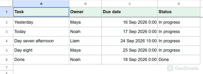
For dates in C and status in D, keep your red overdue rule. Add a second custom rule to the same task range:
=AND(ISNUMBER($C2),$C2>=TODAY(),$C2<TODAY()+8,$D2<>"Done")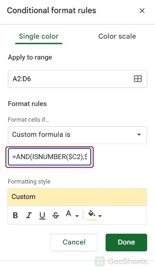
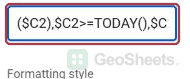
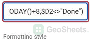
Choose a yellow fill for this rule. It includes today through the seventh day after today, including times on that seventh day.
The red rule checks dates before today, while the yellow rule starts at today. Since these date windows don’t overlap, the same task won’t qualify for both colors.
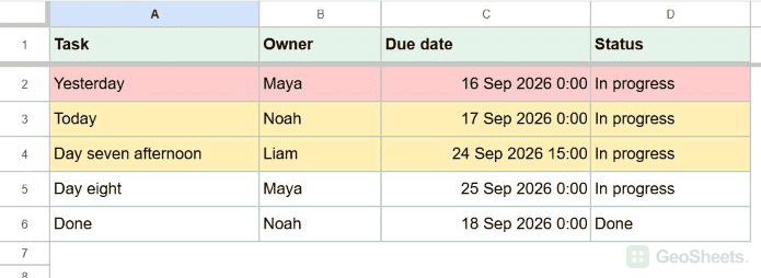
If you use the earlier “include today” red rule instead, the windows overlap. Either move the red rule above the yellow rule or change the yellow rule to begin tomorrow.
Check dates that look overdue but don’t highlight
If an old date stays unhighlighted, first check how Sheets stores it. Applying a date display format doesn’t turn an existing text string into a numeric date value.
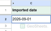
For a suspicious date in C2, enter this formula in a spare cell:
=ISNUMBER(C2)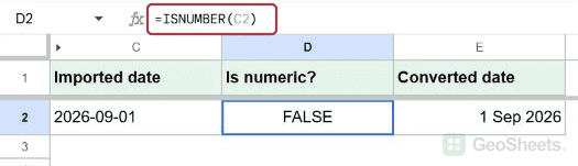
TRUE means the cell contains a number, which a real Sheets date should. FALSE means it’s text, blank, or another nonnumeric value.
If C2 contains a recognizable date stored as text, try converting it in a spare column:
=DATEVALUE(C2)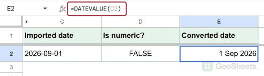
Format the result as a date, then confirm that the day, month, and year are correct before replacing your original values.
Ambiguous text such as 09/10/2026 depends on the spreadsheet’s locale. Don’t assume a successful conversion means the intended date was understood; check the result against your source.
TODAY uses the spreadsheet’s settings. If the date seems a day ahead or behind, check File > Settings, including the time zone and calculation settings.
Google explains those options in its spreadsheet settings guide. TODAY changes when the spreadsheet recalculates; it isn’t a separate reminder or notification service.
Finally, if new tasks appear below the colored range, open the rule and extend Apply to range. For example, change A2:D6 to A2:D100 while keeping the formula’s first row at 2.
Other Google Sheets articles you may also like