Highlight a Row When a Checkbox Is Checked in Google Sheets

If you keep a task list in Google Sheets, checking off a finished task is useful. Having the whole row change color makes completed work much easier to spot as you scan the list.

In this tutorial, I’ll show you how to connect a checkbox to its row’s formatting. We’ll also highlight unfinished tasks, cross out completed ones, and handle rows with more than one checkbox.

Highlight a whole row when its checkbox is checked

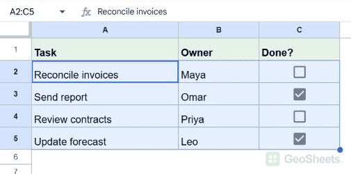
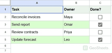
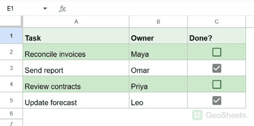
Below, I have a task list in columns A and B, with a Done? column in C. I want the task and owner to change color whenever I check that row’s box.

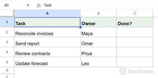
Let’s add the checkboxes first. If your sheet already has them, you can move straight to the formatting steps.

1. Enter your task details in A1:B5 and type Done? in C1.
2. Select C2:C5.

   

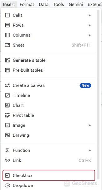
3. Choose Insert > Checkbox. Some English interfaces call this Tick box.

   

   

4. Check C3 and C5 to mark Send report and Update forecast as complete.

   

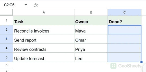
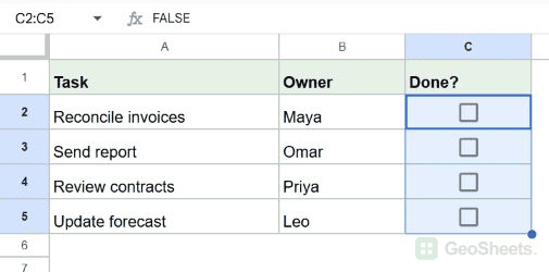
Now let’s make a checked box highlight the task, owner, and checkbox cells in its row.

1. Select A2:C5. Leave the headings out of the selection.

   

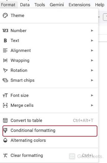
2. Go to Format > Conditional formatting.

   

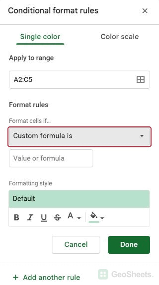
3. Under Format cells if, choose Custom formula is.

   

4. Enter the formula below.
5. Choose a fill color under Formatting style and click Done.

=$C2=TRUE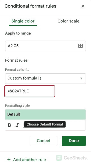

Rows 3 and 5 change color. Reconcile invoices and Review contracts remain unfilled because their boxes aren’t checked.

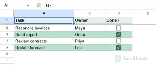
Try unchecking C3. The highlighting on Send report disappears. Check it again, and the highlighting returns. You don’t need to apply a fill color manually each time a task changes.

Why the formula uses $C2

A default checkbox stores TRUE when checked and FALSE when unchecked. Our rule asks whether the checkbox for the current row is TRUE.

The dollar sign locks column C. This keeps the task cell in A and the owner cell in B looking at the same checkbox instead of shifting to neighboring columns.

The row number stays unlocked. Row 2 checks C2, row 3 checks C3, and so on. If you used $C$2, every row would depend on the first checkbox.

If your task list begins on row 5, start the formula with =$C5=TRUE. The first row in your formula must match the first row in Apply to range.

For more examples of fixed and moving references, see the absolute reference guide.

Color only the task details, or include more columns

You don’t have to color the checkbox itself. With tasks in A, owners in B, and checkboxes in C, the same formula can format just the part of the record you want.

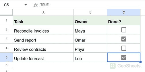
Let’s adjust the existing rule’s coverage.

1. Select a cell in the task list and open Format > Conditional formatting.
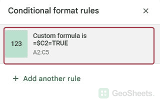
2. Click the checkbox rule.

   

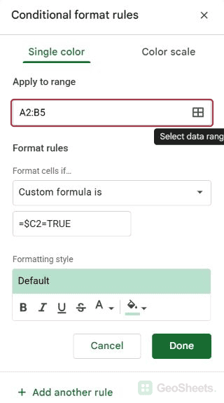
3. Change Apply to range using one of the options below.

   

   

4. Keep =$C2=TRUE as the formula and click Done.

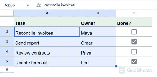
Apply to range	What changes when C is checked
A2:C5	Task, owner, and checkbox cells
A2:B5	Task and owner only
A2:A5	Task name only
C2:C5	Checkbox cell only
A2:F100	All six fields, with room for tasks through row 100

The selected range decides where the style appears. The formula decides which checkbox controls it. Those don’t have to be the same cells.

If you’re extending the list, add checkboxes to the new rows too. Extending a formatting rule doesn’t insert checkbox controls into those cells.

Highlight rows when the checkbox is unchecked

You may prefer to draw attention to work that’s still waiting. For the task list in A2:C5, that means highlighting Reconcile invoices and Review contracts instead of the completed tasks.

I’ll include a check for a task name so empty rows don’t look like unfinished work.

Here are the steps to create an unfinished-task rule.

1. Select A2:C5.

   

2. Open Format > Conditional formatting and choose Custom formula is.

   

3. Enter the formula below.
4. Choose a different fill color, such as pale yellow, and click Done.

=AND($A2<>"",$C2=FALSE)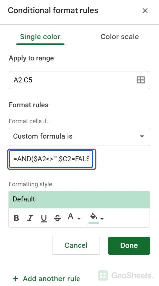

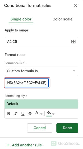
Rows 2 and 4 are highlighted. A completed row doesn’t qualify, and a row without a task name is excluded.

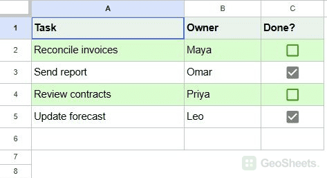
You can keep both this rule and the checked-state rule. They describe opposite checkbox states, so a task moves between the two styles when you check or uncheck it.

This formula assumes the task rows contain default checkboxes. If you’re using custom checked and unchecked values, compare against the actual unchecked value instead, as I’ll show below.

Cross out completed tasks automatically

A fill color isn’t the only way to show completion. If you’d rather cross out the task description when its checkbox is checked, conditional formatting can apply strikethrough for you.

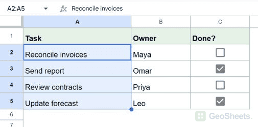
For this example, the task text is in A2:A5 and the checkboxes are in C2:C5. I want the line through the task text without crossing out the owner’s name.

Let’s apply strikethrough just to the task column.

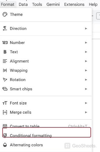
1. Select A2:A5 and open Format > Conditional formatting.

   

   

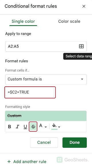
2. Choose Custom formula is.
3. Enter =$C2=TRUE.
4. Under Formatting style, turn on Strikethrough. Choose a muted text color if you want completed tasks to stand out less.

   

5. Click Done.

If you kept the earlier checked-state fill rule, move this strikethrough rule above it in the sidebar. Otherwise, that earlier rule can hide the strikethrough.

Send report and Update forecast appear crossed out. Unchecking either box removes the conditional strikethrough.

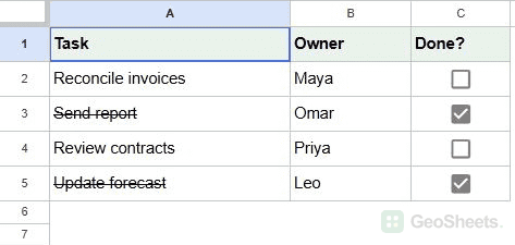
If you also want a fill color on these cells, set it in this rule. Avoid relying on overlapping rules to combine styles; rule order can affect the formatting you see.

Alternatively, apply one rule to A2:B5 and choose both fill and strikethrough there. That crosses out the task and owner together, so pick the range that suits your list.

Use custom checkbox values such as Yes and No

Your spreadsheet may use Yes and No values because other formulas or reports expect that wording. A checkbox can store those values instead of TRUE and FALSE.

Below, we’ll keep the same task layout in A:C, but make each checked box store Yes and each unchecked box store No.

First, change what the checkboxes store.

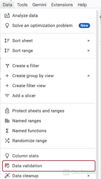
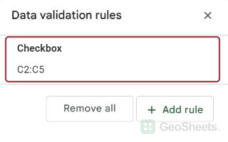
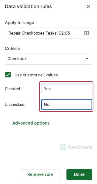
1. Select C2:C5 and open Data > Data validation.

   

2. Open the checkbox rule, or add a rule with Checkbox as its criteria.

   

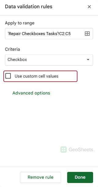
3. Enable Use custom cell values.

   

4. Enter Yes for the checked value and No for the unchecked value, then save the rule.

   

5. Check the boxes for the completed tasks.

   

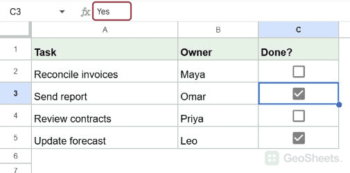
Next, create or edit the conditional-formatting rule for A2:C5 and use this formula:

=$C2="Yes"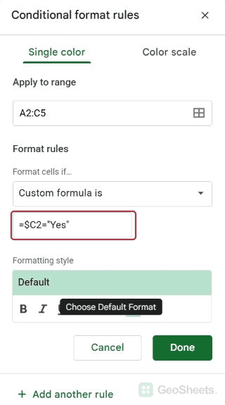

A checked row now qualifies because its checkbox stores Yes. The earlier TRUE comparison no longer describes this setup.

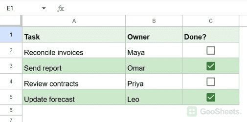
To highlight unfinished named tasks with these custom values, use:

=AND($A2<>"",$C2="No")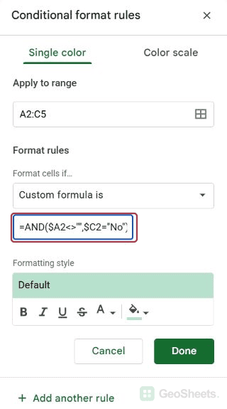

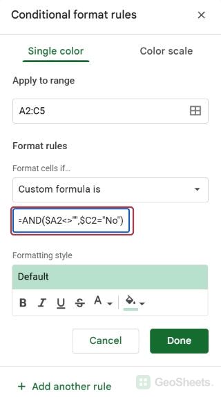
You can confirm the configured values in the data-validation rule. Google’s checkbox documentation also describes the checked and unchecked value settings.

Highlight a row when all its checkboxes are checked

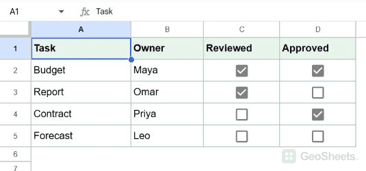
Some tasks need two approvals before they’re complete. Suppose column C records a reviewer’s approval and column D records a manager’s approval. You want a green row only when both are checked.

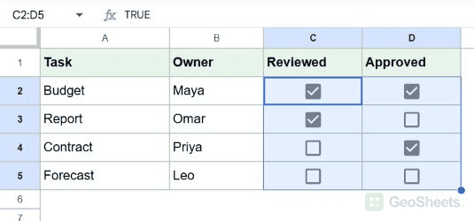
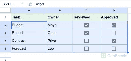
Below, I have that setup in A2:D5, using default TRUE/FALSE checkboxes in C and D.

Let’s require both approvals.

1. Select C2:D5 and choose Insert > Checkbox if those controls aren’t already present.

   

2. Set the checked states shown above.
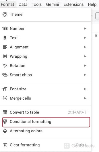
3. Select A2:D5 and open Format > Conditional formatting.

   

   

4. Choose Custom formula is, enter the formula below, select green fill, and click Done.

=AND($C2=TRUE,$D2=TRUE)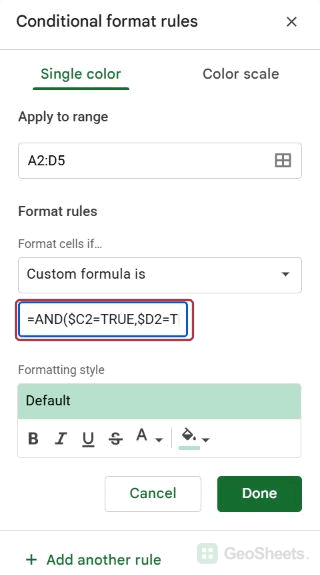

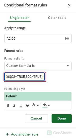
Only the Budget row is highlighted. Report and Contract each have one approval, which isn’t enough for this rule.

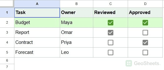
AND requires both checkbox comparisons to be true. To include a third required checkbox in E, add $E2=TRUE as another condition and include E in the applied range if needed.

Highlight a row when any checkbox is checked

For the same two-approval layout, you might instead want to see tasks where approval has started. That means highlighting a row when either C or D is checked.

Use the Budget, Report, Contract, and Forecast example above, with task details in A:B and default checkboxes in C:D.

Let’s change the rule to accept either checkbox.

1. Select A2:D5 and open Format > Conditional formatting.

   

   

2. Edit the all-checkboxes rule if you’re replacing it.
3. Choose Custom formula is and enter the formula below.
4. Select a fill color and click Done.

=OR($C2=TRUE,$D2=TRUE)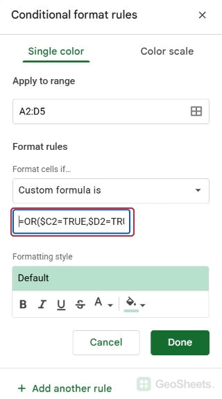

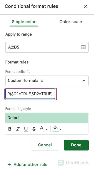
Budget, Report, and Contract are highlighted. Forecast remains unfilled because neither approval is checked.

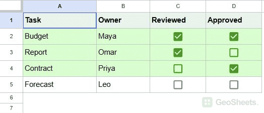
OR needs only one true condition. It also includes rows where both checkboxes are checked, so don’t use it to mean “exactly one approval.”

If you keep a green all-approved rule and a yellow any-approved rule, put the green rule above the yellow one. Fully approved rows satisfy both, and the first matching rule controls their style.

For other combinations, such as a checked box plus a high priority, see conditional formatting with multiple conditions.

Other Google Sheets articles you may also like

• Highlight a Row Based on Another Cell
• Absolute References in Google Sheets
• Conditional Formatting in Google Sheets
• Count checked checkboxes in Google Sheets
• Calculate a total from checked rows in Google Sheets