How to Use Conditional Formatting in Google Sheets

When you’re working with a long list of scores, expenses, or tasks in Google Sheets, it’s easy to miss the entries that need your attention.

Conditional formatting helps those entries stand out automatically. You can highlight low scores, color completed tasks, or shade a range of numbers without manually updating the colors whenever your data changes.

In this tutorial, I’ll show you how to create those rules, choose between simple conditions and formulas, and manage the formatting as your sheet grows.

Highlight numbers with a built-in condition

Let’s start with a simple example. Below, I have five scores in B2:B6, and I want to highlight anything below 80.

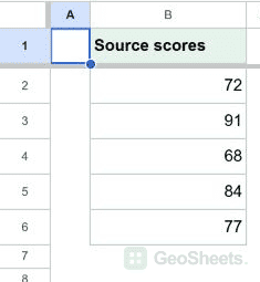
Here are the steps to apply a red fill to the lower scores.

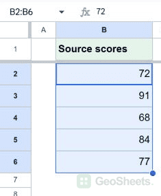
1. Select B2:B6.

   

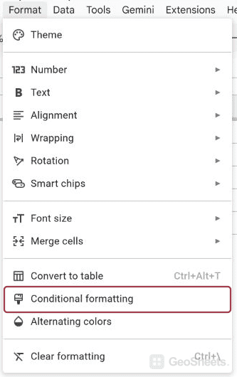
2. Go to Format > Conditional formatting. The rules sidebar opens on the right.

   

3. On the Single color tab, open Format cells if and choose Less than.

   

4. Enter 80 in the value field.

   

5. Under Formatting style, choose a red fill.

   

6. Click Done.

   

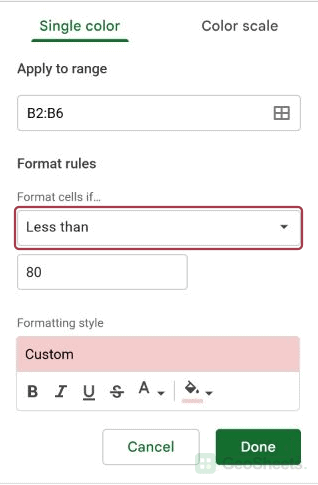
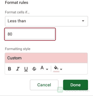
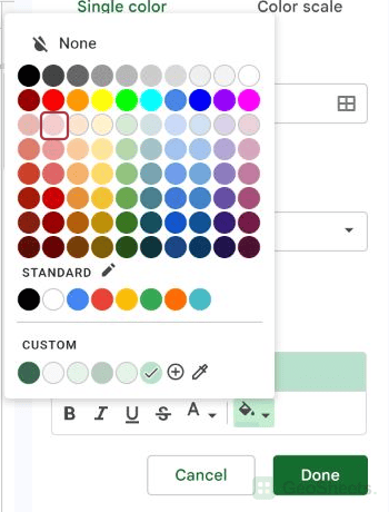
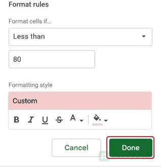
The scores 72, 68, and 77 are highlighted. The scores 91 and 84 remain unchanged because they aren’t below 80.

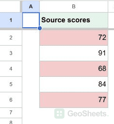
Try changing 72 to 85. Its conditional highlight disappears because the value no longer meets the rule. Changing it back to 72 brings the highlight back.

If your scores are stored as percentages, enter 80% or 0.8 instead of 80. Sheets stores 80% as 0.8, so the comparison needs to use the same scale.

You can also choose Greater than, Is equal to, or Is between. For a fixed pass mark, these built-in conditions are usually simpler than writing a formula.

Highlight cells containing specific text

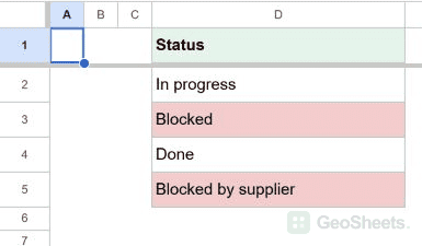
For a status column, text conditions can make exceptions easier to spot. Below, I have four entries in D2:D5: In progress, Blocked, Done, and Blocked by supplier.

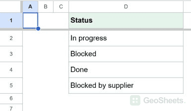
I want both blocked entries highlighted, including the longer description. Here’s how to do that.

1. Select D2:D5, then choose Format > Conditional formatting.

   

   

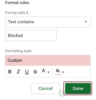
2. Choose Text contains under Format cells if.

   

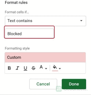
3. Enter Blocked.

   

4. Choose a red fill and click Done.

   

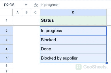
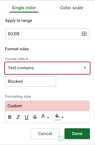
Blocked and Blocked by supplier are highlighted. “Contains” allows the matching text to appear within a longer entry.

If you only want the cell containing Blocked, edit the rule and choose Text is exactly instead. The longer description will no longer qualify.

This distinction matters when labels share words. For example, Text contains “Paid” can also match “Unpaid.” Use an exact match when the entire status must agree.

For several search terms, case-sensitive matching, or a search phrase you can change from a cell, see highlighting cells that contain specific text.

Highlight dates before today

If you have a simple deadline list, you can highlight past dates without writing a formula. For this example, I have yesterday, today, and tomorrow in C2:C4 as actual dates.

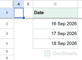
Let’s highlight the date that has already passed.

1. Select C2:C4 and choose Format > Conditional formatting.

   

   

2. Choose Date is before.

   

3. Choose today as the comparison date.

   

4. Choose a fill color, then click Done.

   

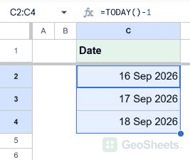
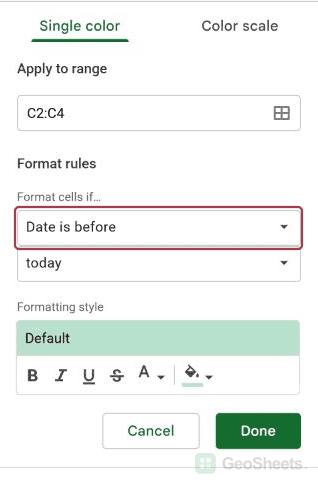
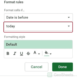
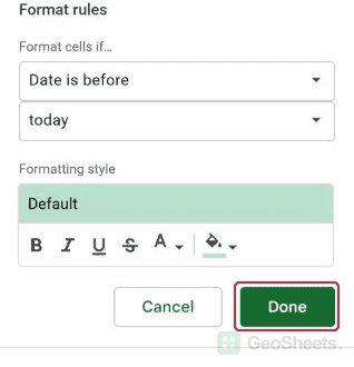
Only yesterday’s date qualifies. Today is not before today, so it remains unchanged.

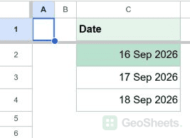
This rule checks dates only. It will still highlight an old deadline belonging to a finished task, because it doesn’t check a Status column.

If you need to exclude completed work or use checkboxes, I’ve covered those variations in the guide to highlighting overdue dates.

Use a color scale to compare numbers

A cutoff tells you which numbers pass a test. A color scale is more useful when you want to see how all the numbers compare.

Below, I’ve copied the scores 72, 91, 68, 84, and 77 into C2:C6. Let’s use a light-to-dark green scale so the higher scores stand out.

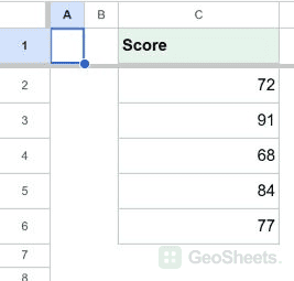
Here are the steps to add the gradient.

1. Select C2:C6.

   

2. Open Format > Conditional formatting.

   

3. Choose the Color scale tab.

   

4. Choose a white-to-green preset, or set the minimum color to white and maximum color to green.

   

5. Leave the endpoints based on the minimum and maximum values in the range, then click Done.

   

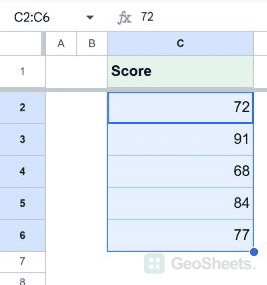
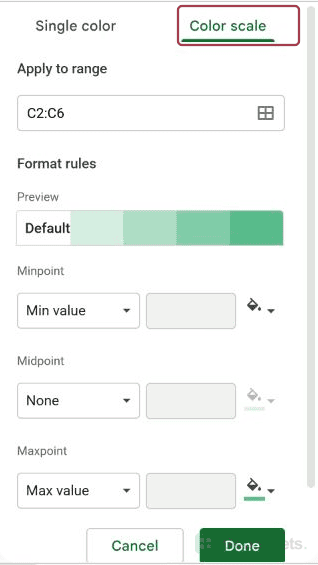
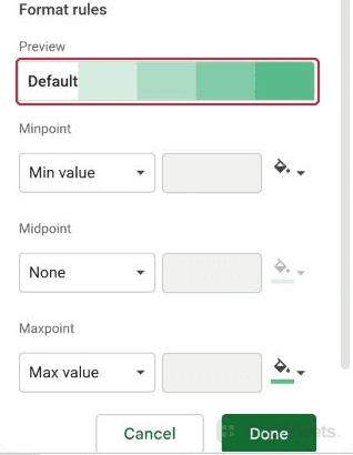
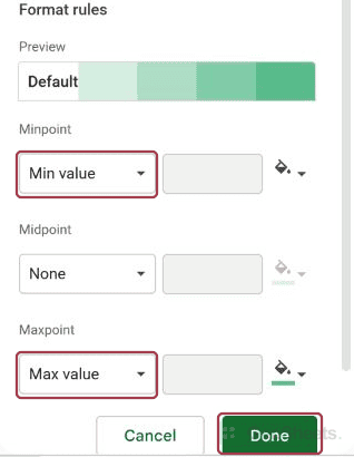
The lowest score, 68, gets the lightest shade. The highest, 91, gets the darkest green. The other scores receive shades between those endpoints.

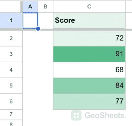
These colors describe the selected group. If you replace 91 with 150, the maximum changes and the other shades adjust relative to the new range.

Keep the same colors across separate reports

If you compare two classes or two months, an automatically chosen maximum can be misleading. The darkest cell in one report may represent a lower score than the darkest cell in another.

To make the colors comparable, edit the scale and set Minpoint to a Number of 0 and Maxpoint to a Number of 100.

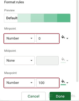
Now both reports use the same endpoints. You can also add a numeric midpoint, such as 80, and choose a middle color when that value has a useful meaning.

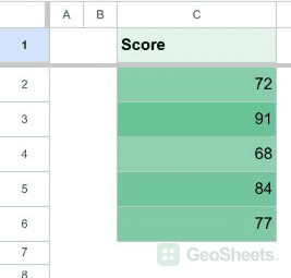
For response times or costs, lower numbers may be better. Reverse your color choices when a dark green maximum would send the wrong message.

Highlight an entire row based on one cell

Sometimes coloring the status cell isn’t enough. You may want the task name, owner, and deadline to change color together when a task is finished.

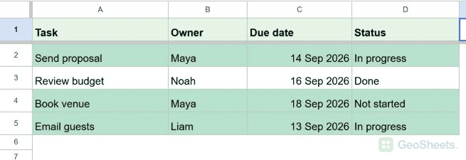
Below, I have a task list in A1:D5. Status is in column D, and Review budget is the only task marked Done.

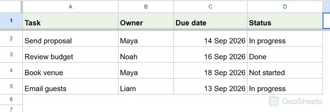
Let’s make the completed task’s entire row green.

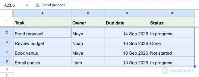
1. Select A2:D5, including every column you want colored.

   

2. Choose Format > Conditional formatting.

   

3. Under Format cells if, choose Custom formula is.

   

4. Enter the formula below.
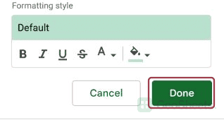
5. Choose a green fill, then click Done.

   

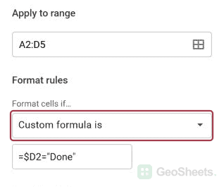
=$D2="Done"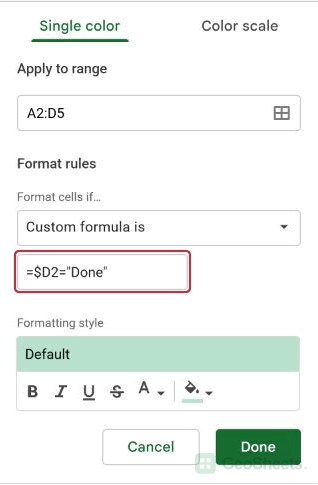

Cells A3:D3 are highlighted because D3 contains Done. The other task rows stay unchanged.

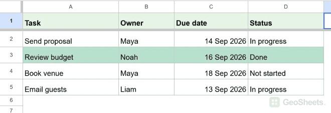
The formula checks whether the status matches Done. When that comparison is TRUE, Sheets applies the chosen style to the cells in that row.

The dollar sign keeps the check in column D as Sheets moves across the row. Leaving the row number unlocked lets each task check its own status.

Reference	Meaning in this example
$D2	Always check column D, using the current row
$D$2	Always check D2, even on other rows
D2	Allow both the checked column and row to shift

If your selected range starts at row 5, your formula must start with $D5. The formula is written for the first row of the range, then adjusted for the rows below it.

To color only task names, change Apply to range to A2:A5. To highlight Blocked tasks instead, change Done to Blocked inside the quotation marks.

The same idea works for completion checkboxes. With default checkboxes in D2:D5, use =$D2=TRUE to highlight checked rows.

For checkbox setup and unchecked-state variations, see formatting rows when a checkbox is checked.

Combine requirements in a custom formula

A task may need to meet two requirements before you want it highlighted. For example, you might want unfinished work belonging to Maya, rather than all of Maya’s tasks.

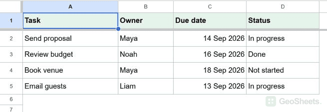
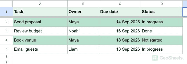
Using the task list above, with Owner in B and Status in D, apply this custom formula to A2:D5:

=AND($B2="Maya",$D2<>"Done")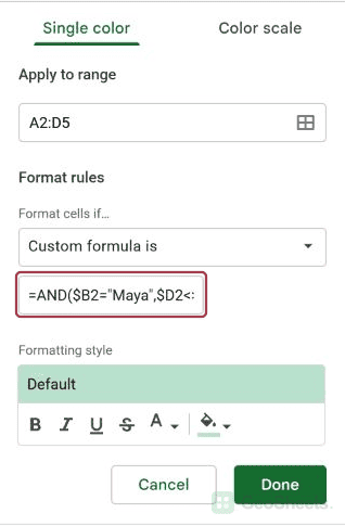

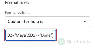
Send proposal and Book venue qualify. AND requires both checks to be true: the owner is Maya, and the status is not Done.

To highlight tasks belonging to Maya or Liam, use OR instead:

=OR($B2="Maya",$B2="Liam")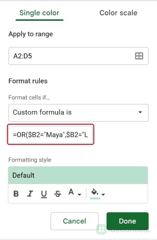

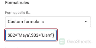
Now Send proposal, Book venue, and Email guests qualify. At least one owner comparison must be true.

You can combine text, numbers, and dates this way. The multiple-condition formatting guide walks through mixed AND/OR logic and changing thresholds.

Highlight repeated entries in a list

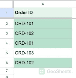
Custom formulas can also compare a cell with the rest of a list. Below, I have order IDs in A2:A6: ORD-101, ORD-102, ORD-101, ORD-103, and ORD-102.

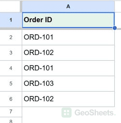
I want every occurrence of a repeated ID highlighted, so I can review the related orders.

Here’s how to add that rule.

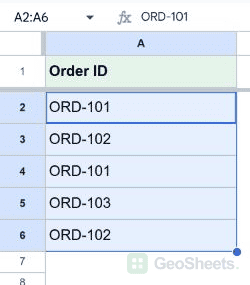
1. Select A2:A6 and choose Format > Conditional formatting.

   

   

2. Choose Custom formula is.

   

3. Enter the formula below, choose a fill color, and click Done.

   

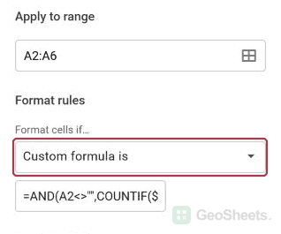
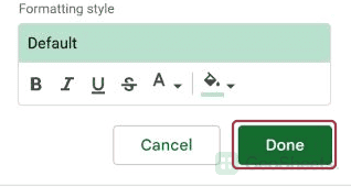
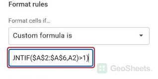
=AND(A2<>"",COUNTIF($A$2:$A$6,A2)>1)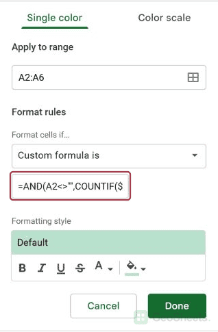

Both ORD-101 entries and both ORD-102 entries qualify. ORD-103 appears once, so it stays unchanged.

COUNTIF counts the current ID within the fixed list. The greater-than-one comparison identifies repeats, and the first condition prevents blank cells from being highlighted.

This highlights duplicates; it doesn’t remove them. For comparing two lists or highlighting only later occurrences, see highlighting duplicate values.

Control which rule takes priority

When two rules can color the same cell, their order matters. Let’s return to scores and use two conditions on B2:B6.

Suppose you want scores below 80 in yellow, but scores below 70 in red. The value 68 meets both conditions.

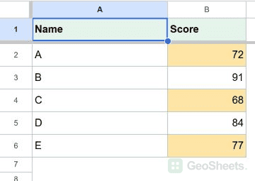
Here’s how to make the stronger alert take priority.

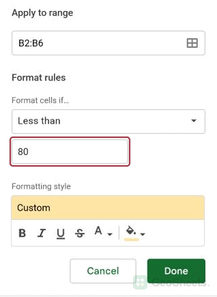
1. Create a Less than 80 rule with a yellow fill on B2:B6.

   

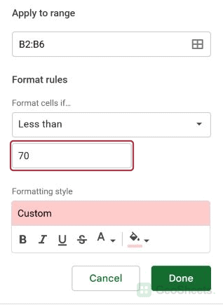
2. Click Add another rule and create a Less than 70 rule with a red fill on the same range.

   

3. In the rules list, drag the Less than 70 rule above the Less than 80 rule.

   

   

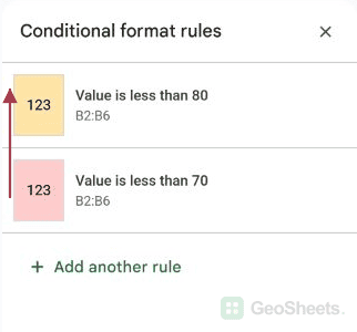
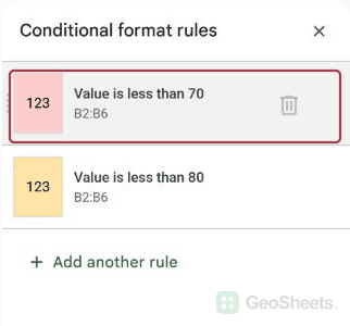
Now 68 is red, while 72 and 77 are yellow. The first matching rule determines the format, as explained in Google’s conditional formatting documentation.

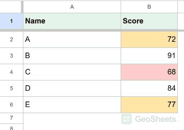
If the yellow rule comes first, 68 receives yellow too. Whenever a correct rule seems to show the wrong color, check the other rules applied to that cell.

Edit, extend, copy, or remove formatting rules

Edit a condition or color

You don’t need to create a new rule each time a threshold changes. Click a cell covered by the rule, open Format > Conditional formatting, and click the existing rule.

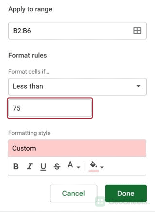
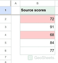
Change the condition, comparison value, or formatting style, then click Done. For example, changing Less than 80 to Less than 75 removes the highlight from 77.

Include new rows

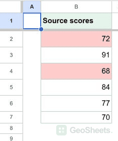
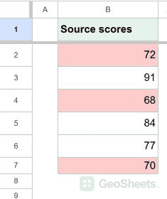
If you add a score in B7 but your rule only covers B2:B6, edit Apply to range to include B7.

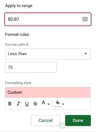
You can reserve room for more data, such as B2:B100. For custom formulas, keep the formula aligned with the first row of the expanded range.

A fixed comparison range inside a formula may also need updating. In the duplicate example, extending only Apply to range won’t expand the COUNTIF range from $A$2:$A$6.

Copy conditional formatting without replacing values

If you want the same rule on another list, Sheets provides a paste option specifically for conditional formatting.

For example, let’s copy the Less than 80 rule from B2:B6 to scores already entered in E2:E6.

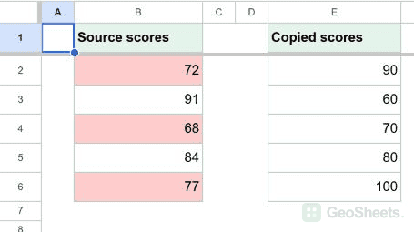
1. Select B2:B6 and copy it.

   

2. Select the top-left destination cell, E2.

   

3. Choose Edit > Paste special > Conditional formatting only.

   

4. Open the destination’s rule and check its range and condition.

   

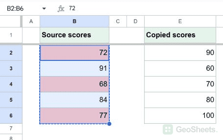
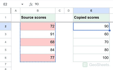
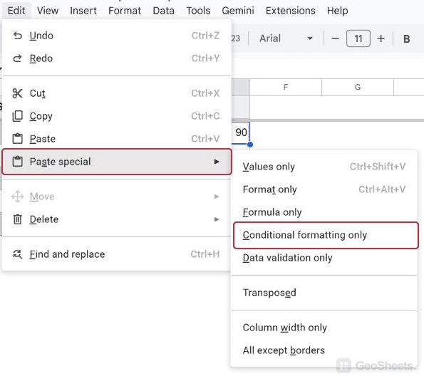
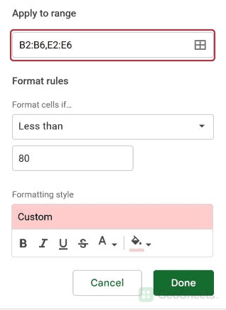
The destination values stay in place while the rule is copied. For a custom formula, inspect its references too: relative references can shift, while references locked with dollar signs stay fixed.

Sheets may add the destination to the existing rule’s applied ranges instead of creating an independent rule. Check that range list before changing or deleting a rule you copied.

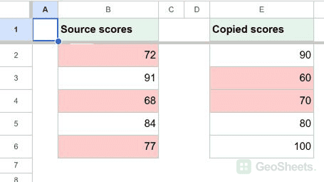
Paste special works within the same spreadsheet file. For another file, recreate the rule there rather than relying on this paste option.

Ordinary copying and pasting can also bring conditional rules with the data. If you only want values, choose Paste values only to avoid importing unwanted formatting.

Remove a rule

To stop a rule from applying, select a cell it covers and open the conditional formatting sidebar. Point to the rule and click its remove icon.

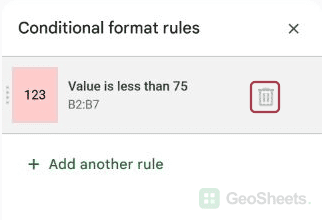
This removes the rule without deleting your data. If a color remains, check whether another rule or a manually applied fill is responsible.

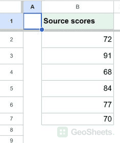
If one rule covers several ranges and you only want to remove formatting from one of them, edit Apply to range instead of deleting the entire rule.

For a rule that still behaves unexpectedly, the conditional formatting troubleshooting guide explains specific range, reference, and data-type problems.

Choose a rule for your next task

Conditional formatting changes how a cell looks when a condition is met. It doesn’t change the value, remove a row, or prevent someone from entering data.

After trying the examples, use these three starting points to choose a rule for another task.

Your goal	Start with	Example
Highlight cells based on their own values	A built-in single-color condition	Scores below 80 or cells containing Blocked
Show how numbers compare with each other	A color scale	A light-to-dark gradient for sales totals
Check another cell or combine requirements	A custom formula	Highlight an entire row when its status is Done

A single-color rule applies the same style to every matching cell. A color scale uses a gradient, so different numbers can receive different shades.

If you only need a one-off manual highlight, you can use the normal fill-color button. Conditional formatting is useful when the highlight should respond to your data.

Other Google Sheets articles you may also like

• Highlight the Highest and Lowest Values in Google Sheets
• Conditional Formatting Across Sheets
• Highlight an Entire Row Based on Another Cell