
If you want to find the mean of a set of numbers in Google Sheets, the AVERAGE function is the quickest way to do it. Point it at a range and it adds the numbers up and divides by how many there are.
In this article, I’ll show you how to use AVERAGE across a few common situations, from a single column of scores to averaging only the rows that meet a condition.
AVERAGE Function Syntax in Google Sheets
The AVERAGE function takes one or more numbers or ranges and returns their mean.
=AVERAGE(value1, [value2, ...])
- value1 is the first number, cell, or range you want to average.
- value2, … are optional additional numbers, cells, or ranges to include.
You can mix individual cells and ranges in the same formula, like =AVERAGE(A2, B2:B10, 50).
When to Use AVERAGE Function
- Finding the mean score, price, or rating across a column of values.
- Averaging numbers spread across several columns in one go.
- Getting a quick class or team average without building a helper column.
- Averaging only the values that pass a condition, by pairing it with FILTER.
- Rounding the result to a tidy number of decimals for reports.
Example 1: Average a Single Column
Let’s start with the most common case, averaging one column of numbers.
Below is the dataset, with student names in column A and their scores in column B, across rows 2 to 7.
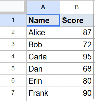
I want the average score for the whole group in cell C2.
Here is the formula:
=AVERAGE(B2:B7)
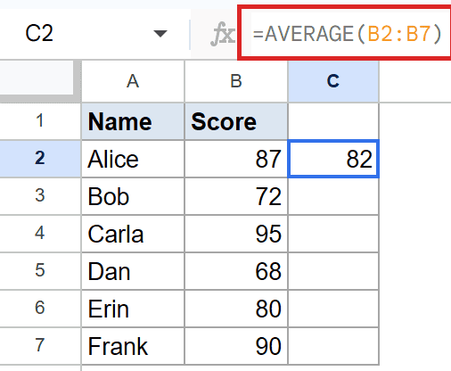
AVERAGE adds up the six scores in B2:B7 and divides by six, the same way the SUM function totals a range before the division step. The result is 82, which is the mean score for the group.
Example 2: Average a Short List of Values
This one works the same way, just on a smaller set of numbers.
Below is the dataset, with product names in column A and their prices in column B, across rows 2 to 6.
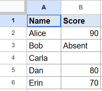
I want the average price of these five products in cell C2.
Here is the formula:
=AVERAGE(B2:B6)
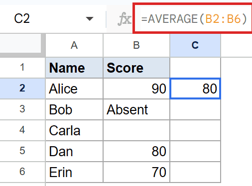
AVERAGE totals the five prices and divides by five. The result is 80, the mean price across the list.
Pro Tip: Blank cells in your range are skipped, not counted as zero. So if one product has no price yet, AVERAGE divides by the number of filled cells, not the full range.
Example 3: Average Across Multiple Columns
You don’t have to stick to one column. AVERAGE will take a block of cells too.
Below is the dataset, with names in column A and two test scores in columns B and C, across rows 2 to 6.
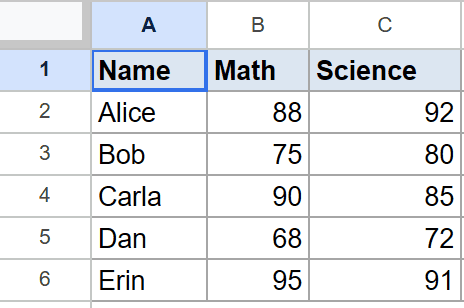
I want the average of every score across both tests in cell D2.
Here is the formula:
=AVERAGE(B2:C6)
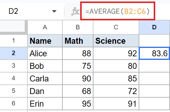
AVERAGE treats the whole block as one pool of numbers. It adds all ten values across the two columns and divides by ten. The result is 83.6.
Example 4: Average Only the Rows That Pass a Condition
Sometimes you only want the average of certain rows. You can do that by feeding AVERAGE a filtered range.
Below is the dataset, with names in column A, a Pass or Fail status in column B, and scores in column C, across rows 2 to 7.
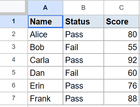
I want the average score of only the students marked Pass, in cell D2.
Here is the formula:
=AVERAGE(FILTER(C2:C7, B2:B7="Pass"))
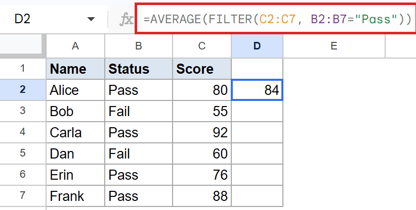
How this formula works:
- FILTER first pulls out only the scores in C2:C7 where column B says “Pass”.
- AVERAGE then takes that shorter list and finds its mean.
- The Fail rows never reach AVERAGE, so they don’t drag the number down. The result is 84.
Pro Tip: If you’d rather average by a condition without FILTER, look at AVERAGEIF. It does the same job in one function when the condition is simple.
Example 5: Average and Round in One Step
Averages often come out with long decimals. You can wrap the whole thing in ROUND to clean it up.
Below is the dataset, with names in column A and scores in column B, across rows 2 to 7.
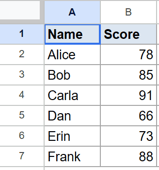
I want the average score rounded to one decimal place in cell C2.
Here is the formula:
=ROUND(AVERAGE(B2:B7), 1)
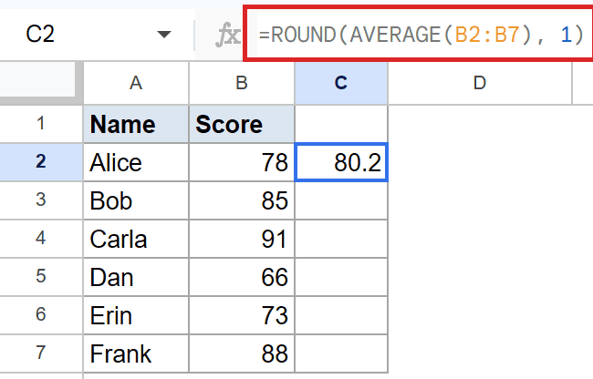
AVERAGE finds the mean first, then ROUND trims it to one digit after the decimal point. The result is 80.2 instead of a long trailing decimal.
Tips & Common Mistakes
- Text and blanks are ignored, not zeroed. AVERAGE only counts numeric cells. A blank or a text label in the range is skipped, so it won’t pull your average toward zero.
- Watch your range edges. If you add a new row below your data, an AVERAGE that ended at B7 won’t include it. Extend the range or use an open range like B2:B.
- An empty range gives an error. If every cell AVERAGE looks at is blank or text, you’ll get a #DIV/0! error because there’s nothing to divide.
That covers the main ways to use AVERAGE in Google Sheets, from a plain column to filtered and rounded results.
Once you’re comfortable with the basic range version, the FILTER and ROUND combinations are easy add-ons for cleaner reports.
List of All Google Sheets Functions
Related Google Sheets Functions / Articles: