Highlight an Entire Row in Google Sheets Based on Another Cell

To highlight an entire row in Google Sheets based on another cell, apply conditional formatting to your full data range and choose Custom formula is. Use a formula such as =$D2="Done".

That rule checks the Status cell in column D and colors the matching row. Below, we’ll build it step by step, then adapt it for an amount threshold and two conditions.

Highlight an entire row when a cell matches specific text

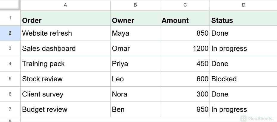
Suppose you have the project list below in A1:D7. Column D holds each project’s status. You want every project marked Done to stand out across all four columns.

Here are the steps to highlight rows where the status is Done:

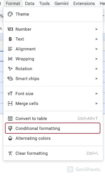
1. Select A2:D7. Leave out row 1 because it contains the headers. You can type A2:D7 into the name box to the left of the formula bar and press Enter.
2. Go to Format > Conditional formatting.

Next, set up the custom formula in the sidebar:

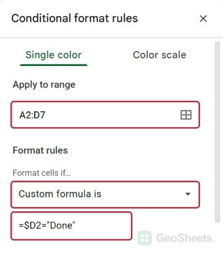
3. In the sidebar, check that Apply to range is A2:D7.
4. Under Format rules, open the Format cells if dropdown and select Custom formula is.
5. Enter the following formula in the formula field.

=$D2="Done"

Under Formatting style, choose a fill color. The example uses the default pale green. Click Done to save the rule.

Rows 2, 4, and 6 are now highlighted: Website refresh, Training pack, and Client survey. The rule colors columns A through D, even though it only checks the value in column D.

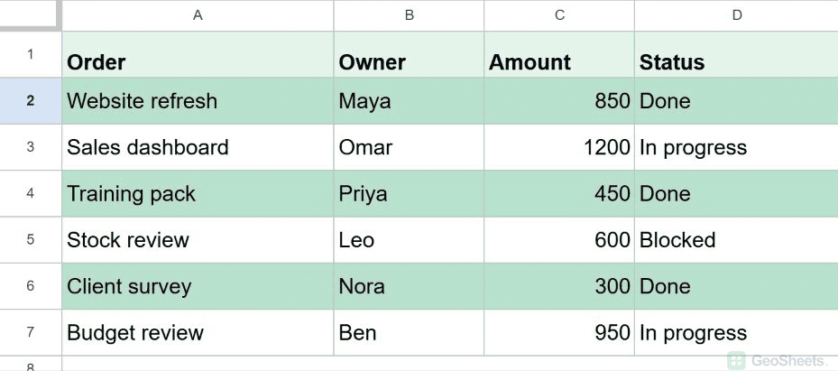
Here, “entire row” means the full width of the selected data range. To include more columns in your own table, widen Apply to range to cover them.

Enter this formula in the conditional formatting sidebar, not in a worksheet cell. The rule changes the appearance of matching cells without replacing their contents.

The comparison checks whether the cell’s value equals Done. It does not search for that word inside a longer status such as Done - awaiting approval. Use the actual status label in your formula.

If column D uses a dropdown, match the option’s stored text in the formula. The dropdown’s chip color is separate from the row’s conditional formatting color.

For a Yes/No status column, our Yes/No dropdown guide explains how to set up consistent options before applying a row rule.

Why the formula uses $D2

The dollar sign before D keeps the rule checking column D as it formats cells across each row. The row number stays relative, so the next row checks D3, then D4, and so on.

The reference starts at row 2 because the selected range starts at row 2. If your data begins at row 5, start the reference at row 5 instead.

Avoid $D$2 for this task. Locking both the column and row makes every selected cell depend on the same D2 value, instead of each row’s own status.

Leaving out the dollar sign before D can shift the checked column as the rule moves across the selected range. Our absolute reference guide explains the different reference types.

If the wrong row changes color, compare the first row in Apply to range with the row number in your formula. If only one cell changes color, check that you selected all the table’s columns.

When an existing rule supplies an unexpected color, inspect the rule order in the sidebar. Google Sheets uses the first true rule for a cell, as explained in Google’s conditional formatting guidance.

Highlight rows when an amount exceeds a number

In this example, the project table occupies A1:D7, and column C contains numeric amounts. The goal is to highlight rows where Amount is greater than 800, regardless of Status.

Here are the steps to highlight rows where the amount exceeds 800:

1. Select A2:D7 and open Format > Conditional formatting.
2. Use a fresh copy of the table, or edit the earlier rule so its colors do not compete with this example.
3. Choose Custom formula is and enter the formula below. Select a fill color and click Done.

=$C2>800

Rows 2, 3, and 7 are highlighted because their amounts are 850, 1200, and 950. Column C is locked; the row number changes for each project.

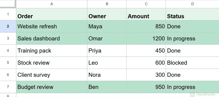
The > operator means strictly greater than. An amount of exactly 800 would not qualify. Enter amounts as numbers, as in this example, rather than text labels containing numbers.

Highlight rows only when two conditions are met

For this version, use a project table in A1:D7 with numeric Amount values in column C and Status in column D. Highlight a row only when Status is Done and Amount exceeds 500.

Here are the steps to highlight rows that meet both conditions:

1. Select A2:D7, then go to Format > Conditional formatting.
2. Work in a fresh copy or replace the previous example’s rule. Choose Custom formula is.
3. Enter the following formula, choose a fill color, and click Done.

=AND($D2="Done",$C2>500)

Only row 2, Website refresh, is highlighted. Its status is Done and its amount is 850. Training pack and Client survey are Done too, but their amounts are below the threshold.

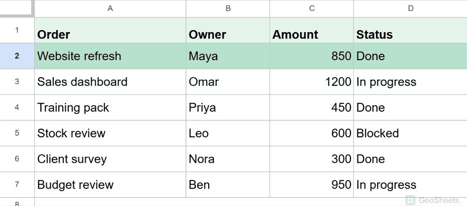
The AND function returns TRUE only when both tests are true. That result tells conditional formatting to apply the chosen color across the row.

Keep the dollar sign before both column letters so each test stays in its intended column. The unlocked row number lets the same rule evaluate every project in the range.

Other Google Sheets articles you may also like

• Use IF to return a result based on a condition
• Fill color options and shortcuts in Google Sheets