
When conditional formatting does nothing in Google Sheets, start with the rule’s range and formula. Most failures happen because the rule evaluates the wrong cells or never evaluates to TRUE.
Use this checklist for a rule that highlights cells, rows, or a status column. It also helps when formatting works on one row but skips others.
Check the Apply to range first
A rule can only format cells included in its Apply to range. If your new rows sit outside that field, the rule may be correct but cannot reach them.
Use these steps to confirm the selected cells.
- Select a cell that should be formatted.
- Choose Format > Conditional formatting.
- In the sidebar, compare Apply to range with the cells you expect to change.
- Edit the range, then choose Done.
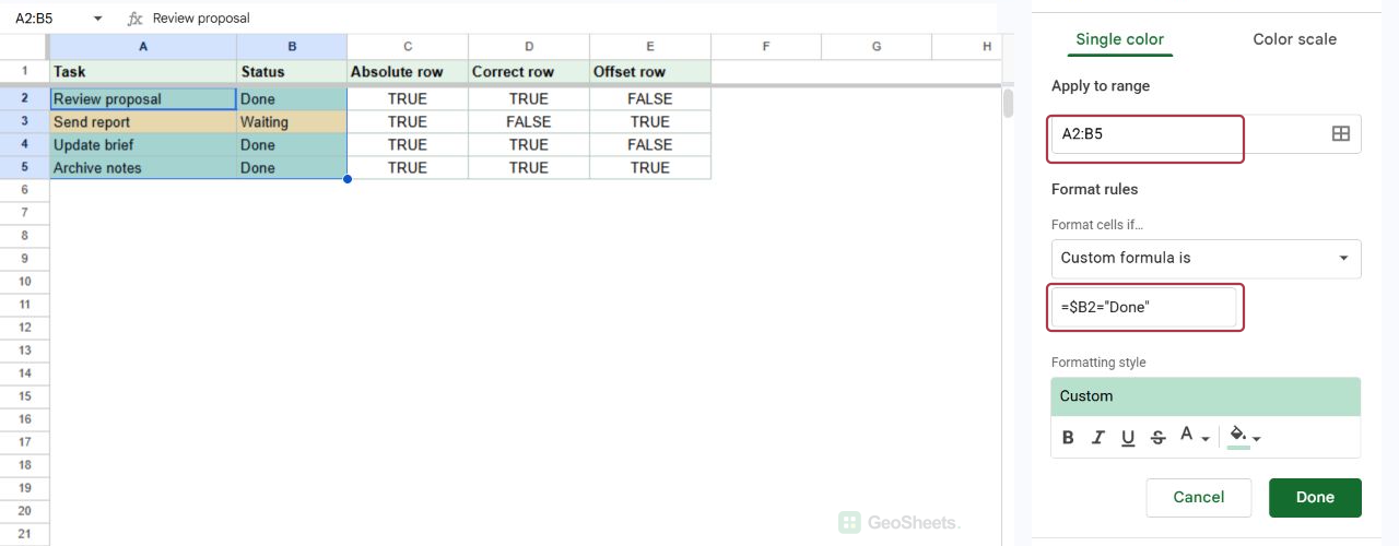
For a whole-row status rule, the range might be A2:B5. A range of B2:B5 would format only the Status cells, even when its formula checks the same values.
Match a custom formula to the first row
A custom formula is evaluated from the upper-left cell of its applied range. Its row reference must match the first data row in that range.
For A2:B5, use =$B2="Done" to format both cells in each row when column B says Done.
The dollar sign locks column B. Leaving the row relative lets Sheets check B2, B3, B4, and B5 as it evaluates each row.
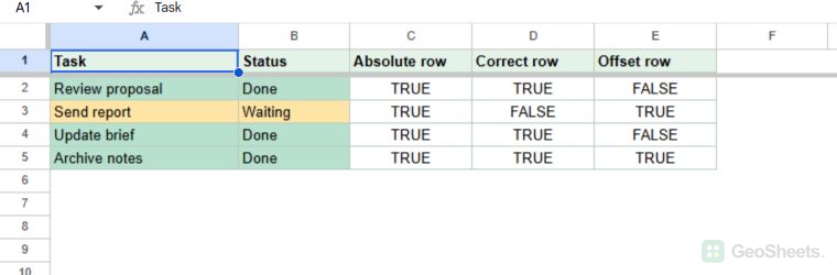
In a tested sheet, that formula highlighted rows 2, 4, and 5. Those were the rows with Done in column B.
These three comparisons show the difference.
| Formula pattern | Observed results in rows 2–5 | What it does |
|---|---|---|
=$B$2="Done" | TRUE, TRUE, TRUE, TRUE | Checks B2 every time. |
=$B2="Done" | TRUE, FALSE, TRUE, TRUE | Checks each row’s status. |
=$B1="Done" | FALSE, TRUE, FALSE, TRUE | Starts one row too high. |
If references still feel confusing, see our guide to the absolute reference shortcut in Google Sheets.
Confirm that the condition can become TRUE
Conditional formatting has no visible error message when its condition is false. Test the condition in an unused cell before assuming the formatting is broken.
For a status rule, enter =$B2="Done" beside the first record. It should return TRUE for a matching status and FALSE for a different one.
Check the actual stored values if it stays FALSE. A trailing space, a different label, or a text value where you expected a number can change the result.
Google’s conditional-formatting guidance also documents text matching and custom formulas. Use the rule type that matches the values you actually store.
Put the rule that should win first
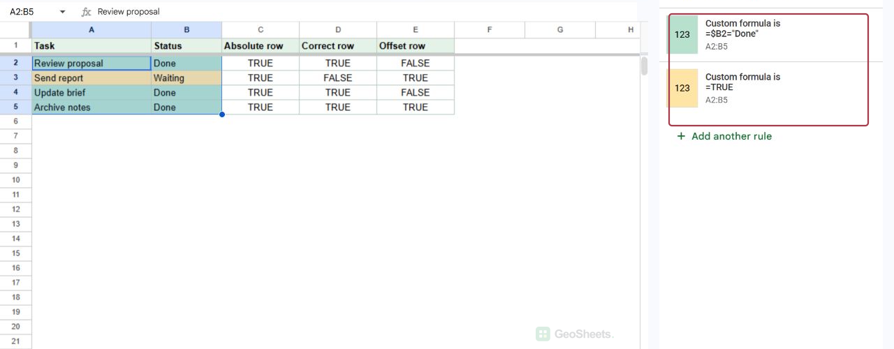
Two rules can both be true for the same cell. Google Sheets uses the first true rule in the sidebar’s list to define the formatting.
Use these steps to inspect an overlap.
- Open Format > Conditional formatting.
- Select a cell with the unexpected color.
- Review every rule whose range includes that cell.
- Move the rule you need first, or make the conditions mutually exclusive.
For example, a broad “not blank” rule can hide a more specific status rule if both match. Keep each range narrow when the rules serve different parts of a sheet.
Retest one row, then extend the rule
Change one part of a rule at a time. First make it work for the top data row, then expand the range and check a matching and nonmatching row.
For row-based formatting, follow the complete setup in Highlight an Entire Row in Google Sheets Based on Another Cell.
If you only need a one-off color rather than an automatic rule, use the fill color options in Google Sheets.
Other Google Sheets articles you may also like