
When several people update a task list, the same status can acquire several spellings. A dropdown gives them a shared set of choices.
We’ll build five versions of a status dropdown, starting with choices typed into the rule. The same three tasks stay visible throughout the examples.
Create a dropdown by typing the options
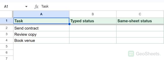
Here is the starting task list. Column A has the task names, and B2:B4 is empty. We want each task to have a status choice.
For a short, fixed list, enter the choices directly in the dropdown rule. Here are the steps:
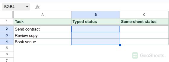
- Select B2:B4, beside the three task names.

Select the destination cells, not the task names. - Open Data > Data validation.

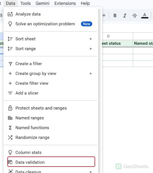
The Data menu contains Data validation. - In the sidebar, click Add rule.

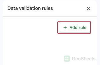
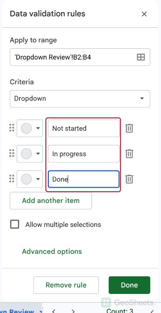
Add a rule for the selected B2:B4 range. - Under Criteria, choose Dropdown. Enter Not started and In progress, then use Add another item for Done.

The rule contains all three typed options. - Click Done. Open B2’s dropdown and choose In progress.

After: B2 contains In progress, and its choices are visible.
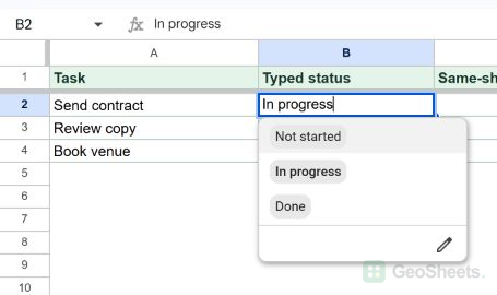
The rule also covers B3 and B4. Each task can have a different selection. You can reach the same setup through Insert > Dropdown or a cell’s right-click menu.
For a simpler two-choice example, see how to add a Yes/No dropdown.
Create a dropdown from cells on the same sheet
This time, the choices live in G2:G4 on the task sheet: Not started, In progress, and Waiting. We’ll use them for C2:C4.
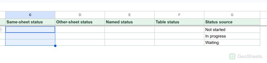
Here are the steps to connect the status cells to that source:
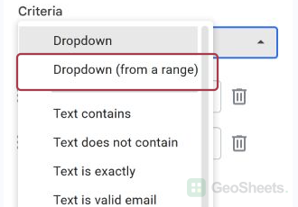
- Select C2:C4. Open Data > Data validation and click Add rule. Under Criteria, choose Dropdown (from a range).

Choose Dropdown (from a range) for the selected C2:C4 cells. - Use the source-range picker to select G2:G4, confirm the range, and click Done. Check that the sidebar previews the three source values before saving.
Apply to range is C2:C4; the source is G2:G4. - Open the dropdown in C2 to check its choices.

After: C2 offers the values from G2:G4.
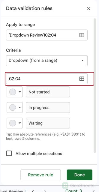
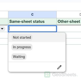
The two ranges have different jobs. Apply to range identifies cells people edit; the field under Criteria identifies cells supplying choices.
Changing Waiting in G4 changes the offered choice. Adding a value in G5 requires extending a fixed G2:G4 source, unless you use a source designed to grow.
Create a dropdown from a list on another sheet
The Dropdown Review Lists tab has Status in A1 and three choices in A2:A4. We’ll use that central list for D2:D4 on the task tab.
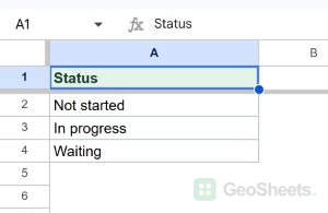
Here are the steps to use that list:
- Return to the task tab and select D2:D4. Open Data > Data validation > Add rule, then choose Dropdown (from a range).

Select D2:D4 beside the tasks before connecting the other tab. - Use the source-range picker to select Dropdown Review Lists!A2:A4. Confirm it and click Done.
The destination rule points to A2:A4 on the separate list tab. - Open D2’s dropdown to verify the three choices.

After: the task tab displays choices from the list tab.
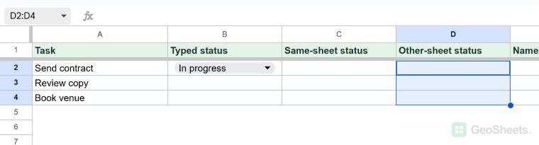
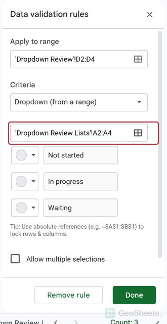
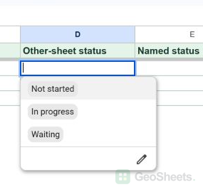
Because the tab name contains spaces, Sheets displays its reference with quotation marks. This source is another tab in the same spreadsheet file.
For choices stored in another file, first bring them into this spreadsheet with IMPORTRANGE. Then validate against the local imported cells.
Create a dropdown using a named range
A name makes a shared list easier to recognize. We’ll call the list tab’s A2:A4 range ReviewStatusOptions and use it for E2:E4.
Here are the steps to name the source and connect the dropdown:
- On the list tab, select A2:A4. Open Data > Named ranges, enter ReviewStatusOptions, check the range, and click Done.

The name ReviewStatusOptions refers to A2:A4 on the list tab. - On the task tab, select E2:E4. Add a Dropdown (from a range) rule and set its source to ReviewStatusOptions. Click Done.
The E2:E4 rule uses the named range as its source. - Open E2’s dropdown to check the available statuses.

After: E2 offers the named range’s values.
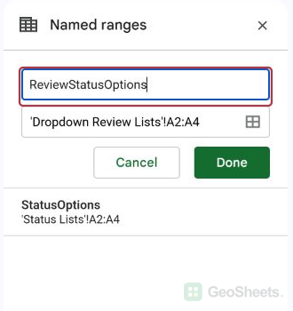
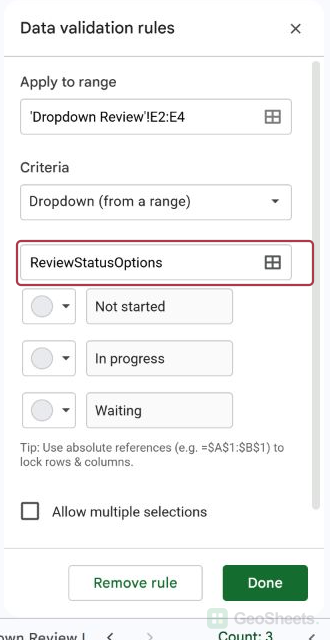
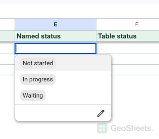
The name points to the source; it does not copy the options. If the list grows past A4, extend the named range in Data > Named ranges.
Range names can contain letters, numbers, and underscores, but no spaces. See Google’s named-range rules.
Create a dropdown from a table column
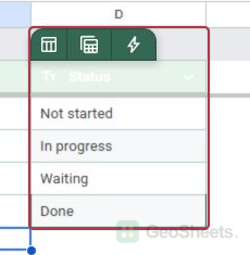
On the Status Lists tab, the StatusChoices table has a Status column. It contains Not started, In progress, Waiting, and Done.
Here are the steps to use that table column for F2:F4:
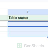
- On the task tab, select F2:F4. Add a Dropdown (from a range) rule.

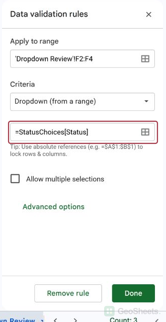
Select F2:F4 as the cells that will receive the table-backed dropdown. - Set the source to
=StatusChoices[Status]and click Done. The first name identifies the table; the name in brackets identifies its column.The F2:F4 rule uses the Status column of the StatusChoices table. - Open F2’s dropdown and choose a status.

After: F2 contains Not started, and the table’s four choices are visible.
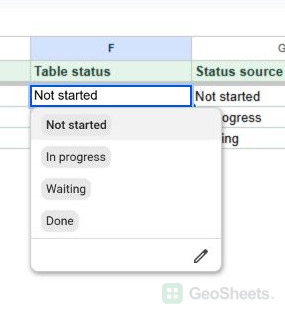
When you add a row inside the table, its new status becomes an option without changing the rule. If it does not appear, check that the row belongs to the table.
To make a source table from ordinary cells, select a range with a header, choose Format > Convert to table, and give the table a clear name.
Choose where your dropdown options will come from
Now that you’ve seen each method, choose based on where you want to maintain the list:
| Source | Useful when | How you update it |
|---|---|---|
| Typed options | The list is short and stable | Edit the rule |
| Cells on this sheet | The list belongs beside the task data | Edit the source cells |
| Cells on another tab | Several tabs share the list | Edit the central list tab |
| Named range | A readable source name helps | Edit its cells or boundary |
| Table column | The source gains new rows | Add a row inside the table |
A dropdown is one type of data validation. Other rules can check numbers, dates, or text without presenting choices.
Edit dropdown options and appearance
Select a dropdown cell, then open Data > Data validation and click its rule. The sidebar shows its destination range and criteria.
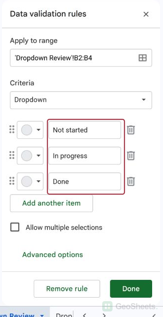
For typed choices, edit the items in the rule. For a range-based list, edit its source cells. To cover more task rows, expand Apply to range.
You can give individual choices colors. Under Advanced options, choose Chip, Arrow, or Plain text for the cell’s appearance.
To color an entire completed row, use conditional formatting based on the status cell.
Choose whether to reject values outside the list
Expand Advanced options in the rule. Under If the data is invalid, choose Reject the input for a strict list or Show a warning for exceptions.
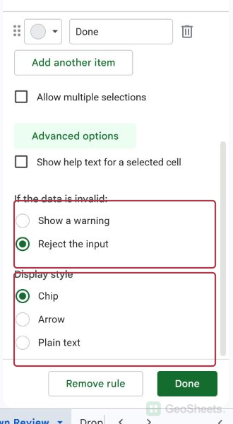
For example, a strict status list rejects Deferred when it is not an option. Warning mode permits it but marks it as outside the list.
Allow more than one selection in a cell
A task should have one status, but it can have several labels. This task list starts with empty label cells in B2:B4.
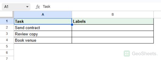
Here are the steps to allow more than one label in a cell:
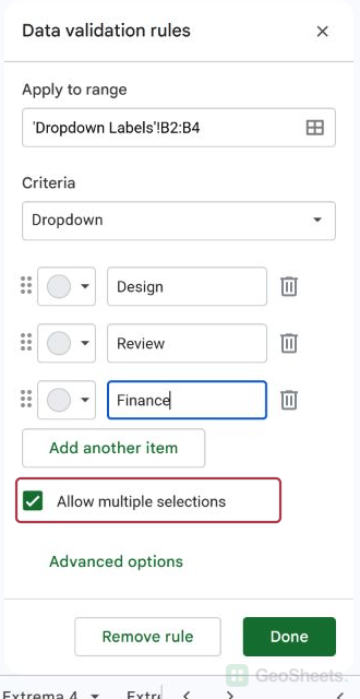
- Select B2:B4. Add a Dropdown rule with Design, Review, and Finance. Keep Chip display and enable Allow multiple selections.
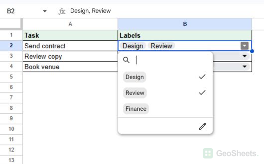
The rule has three labels and allows multiple selections. - Click Done. Open B2’s dropdown and choose Design and Review.

After: B2 contains both Design and Review, checked in the open list.
Multiple selection applies to chip dropdowns on desktop. Google says mobile currently cannot choose several options, even when this setting is enabled. See its dropdown guidance.
Copy or remove a dropdown
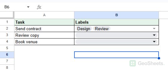
B2 contains two selected labels; B6 is empty. We’ll copy the dropdown choices to B6 without copying B2’s selected labels.
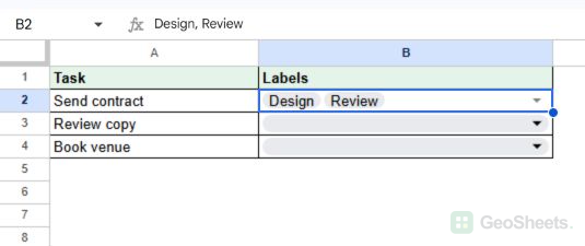
Here are the steps to copy only the validation:
- Select B2 and press Ctrl+C. Then select the empty B6.

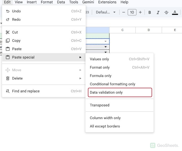
B2 is outlined as the copied source, and B6 is the selected destination. - Choose Edit > Paste special > Data validation only.

Use Data validation only for the selected B6 destination. - Open B6’s dropdown to check the result.

After: B6 has the three choices but no copied label value.
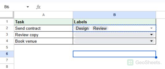
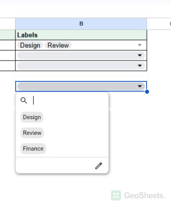
In this example, Sheets added B6 to the same rule’s Apply to range as B2:B4. To remove only B6, open the rule and remove B6 from that field.
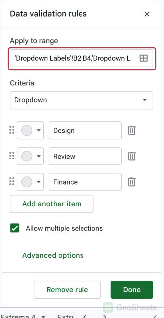
After saving the shortened range, B6 no longer has a dropdown, while B2:B4 still do. Use Remove rule only when you want to remove every destination covered by that rule.
Other Google Sheets articles you may also like