
Use a custom formula when a formatting rule should check more than one thing. The formula returns TRUE only for rows that meet the combination of conditions you define.
Use AND when every condition must match. Use OR when any condition can match. Lock the columns you are checking, but leave the row number relative.
When a custom formula is the right tool
Built-in formatting conditions check each cell by itself. A custom formula is more useful when a task row should depend on values in two or more columns.
For example, a project tracker may need a highlight only when Priority is High and Status is In progress. Formatting either condition alone would show too many rows.
Apply the rule to the cells you want to style, then write the formula for the first row of that applied range. Sheets adjusts relative row references for each later row.
Format rows when all conditions are true
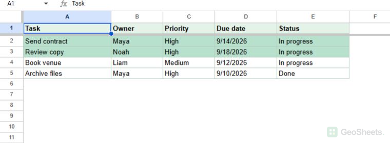
This example highlights high-priority tasks that are still in progress. The source data has Task, Owner, Priority, Due date, and Status in columns A through E.
=AND($C2="High",$E2="In progress")AND returns TRUE only when both tests return TRUE. The dollar signs keep Sheets in columns C and E while the row number moves from row 2 to row 3 and beyond.
In the verified fixture, Send contract and Review copy were both High and In progress. Those two rows were formatted; the Medium task and the completed High task remained unchanged.
Use these steps to apply the same rule to a task list.
- Select the output range, such as
A2:E5. Leave out the header row unless you want it formatted too. - Choose Format > Conditional formatting.
- Under Format cells if, choose Custom formula is.
- Enter
=AND($C2="High",$E2="In progress"). - Choose a fill or text style, then click Done.
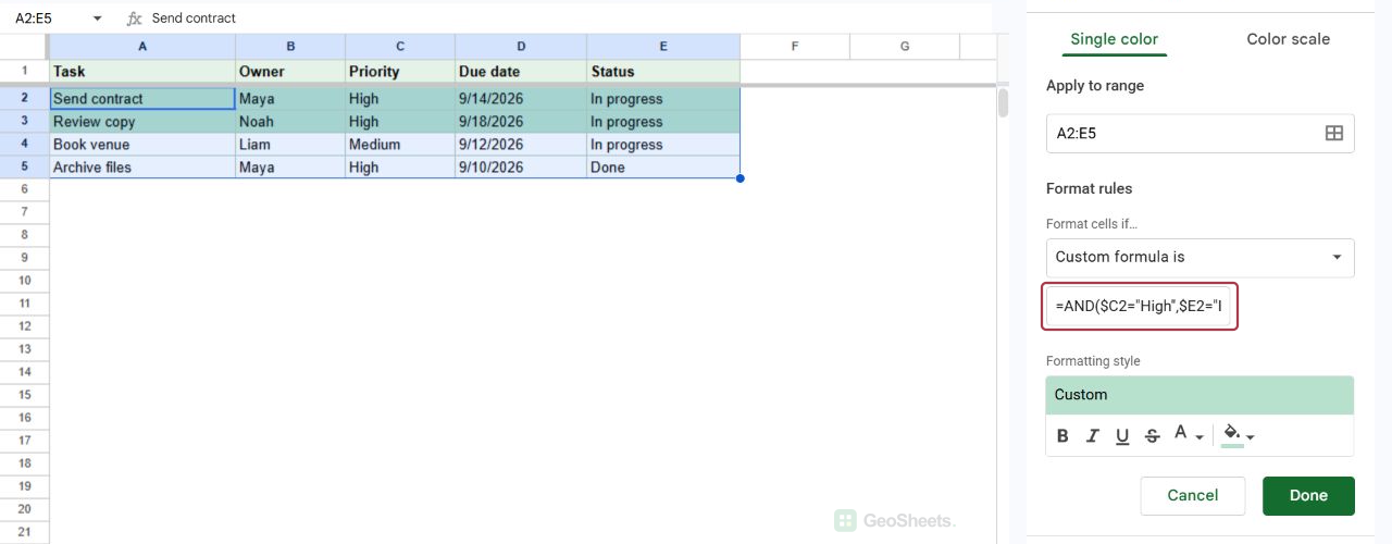
Match the first row. The formula must use the first data row in your applied range. If the range starts at row 2, start each moving reference with 2.
For the full setup of formatting a row from one controlling cell, see how to highlight an entire row based on another cell.
Use OR when either condition can match
Use OR when one matching condition is enough. For example, you may want to highlight a task that is High priority or Blocked.
=OR($C2="High",$E2="Blocked")This rule returns TRUE for a High task, a Blocked task, or a row that is both. It returns FALSE only when neither test is true.
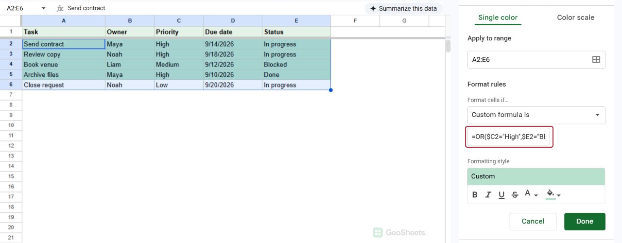
In the live fixture, this rule highlighted both High tasks, the Blocked Medium task, and the completed High task. The Low task that was still in progress remained unchanged.
Choose the correct references
Use $C2 when every formatted row should check its own Priority value in column C. The column stays fixed while the row changes as Sheets evaluates the range.
Using $C$2 would make every row check the same Priority cell. That is useful only when one fixed control cell should govern the whole range.
Keep all formatting formulas on the same sheet when possible. Google documents same-sheet custom-formula references directly; cross-sheet rules need a separate approach and should be tested carefully.
Keep multiple rules manageable
Give each rule one clear job. A rule for High and In progress is easier to inspect than a long formula that mixes unrelated status, date, and owner tests.
When results look wrong, compare the applied range with the formula’s first row. Then inspect the sidebar for another rule that styles the same cells.
The AND function in Google Sheets is also useful outside formatting when a formula needs one TRUE or FALSE result from several tests.
Other Google Sheets articles you may also like