
To add amounts only from checked rows, use SUMIF. The formula checks the checkbox column and adds the matching amounts from another column.
The total changes when you check or uncheck a row. If your checkboxes store custom words, use the configured checked word as the criterion.
Add amounts from checked rows with SUMIF
This expense list has checkboxes in column B and amounts in column C. Printer paper, shipping labels, and packing tape are checked; folders and markers are not.
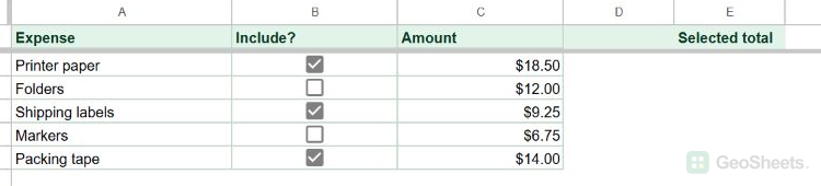
Use the checkbox column as the condition for the expense total.
1. Click E2, outside the expense list. Enter the formula:
=SUMIF(B2:B6,TRUE,C2:C6)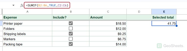
B2:B6 tells SUMIF which cells to check. TRUE means a default checkbox is selected. C2:C6 supplies the amounts to add.
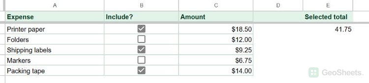
Press Enter and move the selection off E2. The checked rows total 41.75: 18.50 + 9.25 + 14.00.
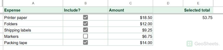
2. Check the box for Folders in B3. That adds its 12.00 amount, so the total becomes 53.75.
The checkbox range and amount range must cover the same rows. If you add expenses, extend both ranges together so every checkbox still lines up with its amount.
If the total stays at zero despite visible checkmarks, inspect whether the checkbox rule uses custom values. A checked box storing text will not match the default TRUE criterion.
Use a custom checked value in SUMIF
In a second expense list, the checkbox rule stores Approved for checked and Hold for unchecked. The checked rows are the same three expenses.
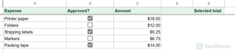
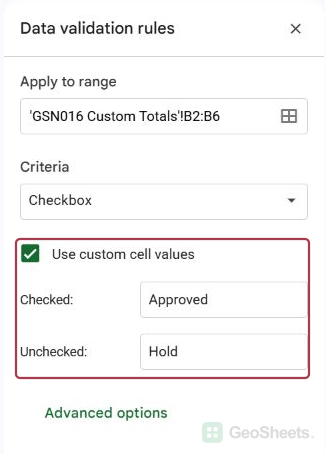
Use the custom checked word to total these approved expenses.
1. Click E2 and enter the configured checked word in quotation marks:
=SUMIF(B2:B6,"Approved",C2:C6)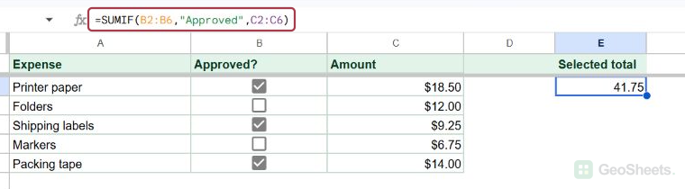
Press Enter and move the selection away. The three approved expenses total 41.75.
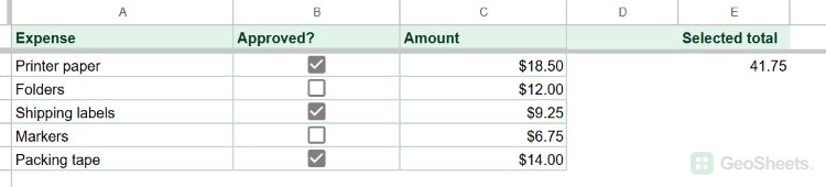
Match the criterion to the value stored by your rule. For example, a rule with Yes as its checked value needs "Yes" in the formula.
Google’s SUMIF documentation explains the criterion and sum ranges. Its checkbox guide shows how custom checked and unchecked values work.
Other Google Sheets articles you may also like