
Use a custom conditional-formatting formula to flag tasks with a due date before today. Add checks for blank dates and completed tasks so they stay out of the alert.
The formula can color only the due-date cell or the whole task row. This guide uses a four-column task list and highlights the entire row.
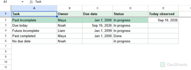
Highlight incomplete tasks with past due dates
Apply the rule to the rows you want to color. In this example, due dates are in column C and task status is in column D.
The following steps create one rule that matches an incomplete task only when its due date is earlier than the current date.
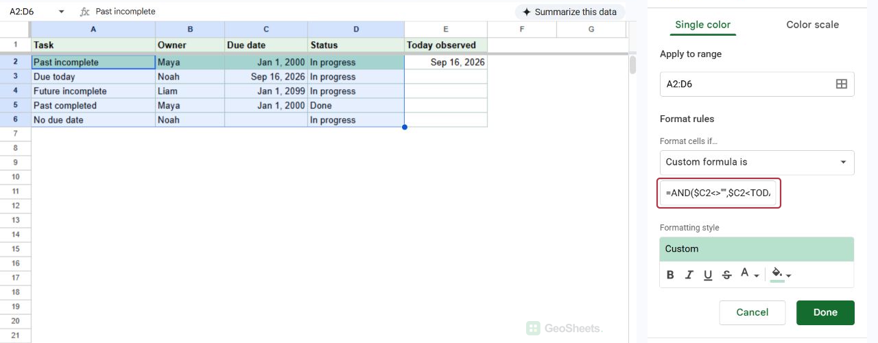
- Select the task range, such as
A2:D100. - Choose Format > Conditional formatting.
- Under “Format cells if,” choose Custom formula is.
- Enter
=AND($C2<>"",$C2<TODAY(),$D2<>"Done"). - Choose a fill color and select Done.
The tested rule uses row 2 because it is the first row of the selected range. The dollar signs keep the due-date and status columns fixed as Sheets evaluates each row.
$C2<>"" requires a due date. $C2<TODAY() identifies a past date, and $D2<>"Done" excludes finished work.
Read more about the TODAY function if you need to understand how Sheets supplies the current date.
Format the date cell or the whole row
The applied range controls what changes color. The formula can stay the same when you change the range.
Use these range choices to match the way people scan your sheet.
- Select
C2:C100to highlight only the due-date cells. - Select
A2:D100to highlight each full task row. - Start the formula with the first row of the selected range, such as row 2 for either example.
A full-row format helps when the task name and owner matter as much as the date. A date-only format keeps a dense project sheet quieter.
Include today when your process calls it overdue
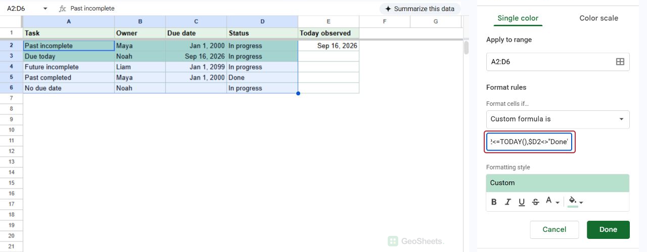
The tested formula uses <TODAY(), so a task due today does not match. That suits a process where today remains available until the day ends.
If your team treats a task due today as urgent, use this variation instead.
=AND($C2<>"",$C2<=TODAY(),$D2<>"Done")The added equals sign makes today match. This variation is documented here for adaptation and was not separately tested in the fixture.
Make sure the due date is a real date
Conditional formatting compares date values, not a date-shaped label. A copied value that looks like a date can still be text.
Try changing the date cell to a standard date format. If it still does not match, convert the source value with DATEVALUE in a helper column before applying the rule.
The current date also depends on the spreadsheet time zone. Check File > Settings when a deadline appears to cross at the wrong local time.
Keep the rule practical in large task lists
TODAY() is volatile, so Sheets recalculates it as the workbook updates. Keep the applied range close to your real task list instead of formatting entire columns.
Other Google Sheets articles you may also like