
ASIN returns the inverse sine of a number in Google Sheets. For a right triangle, use the opposite-side length divided by the hypotenuse to find an angle.
The result is in radians. Wrap ASIN in DEGREES when you want a degree measurement, and keep the input between -1 and 1 inclusive.
ASIN function syntax
=ASIN(value)- value: a number from -1 through 1, or a reference to that number.
The Google ASIN reference describes the function arguments.
Example data
Enter this dataset starting in A1. Leave cells marked “leave empty” empty; type any displayed formula as a formula. Keep a separate blank area for the results.
| Ratio | Meaning |
|---|---|
| 0.5 | Opposite ÷ hyp. |
| -1 | Lower boundary |
| 0 | Zero |
| 1 | Upper boundary |
| 1.2 | Invalid |
The examples below use this dataset unless the formula supplies its own values. Array results need enough empty cells to expand. The formulas use commas as argument separators. Your spreadsheet locale may require semicolons.
Find an angle in radians
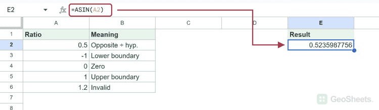
An opposite-to-hypotenuse ratio of 0.5 gives approximately 0.5236 radians. ASIN returns the angle, not another side-length ratio.
=ASIN(A2)Result: 0.5235987756
Return the angle in degrees
DEGREES converts the radian output to 30 degrees. Apply the conversion after ASIN; its input is a ratio, not an angle.
=DEGREES(ASIN(A2))Result: 30
This ratio corresponds to 60 degrees. ROUND removes an insignificant floating-point display difference.
=ROUND(DEGREES(ASIN(SQRT(3)/2)),2)Result: 60
Check the allowed boundaries
The lower input boundary -1 returns -π/2 radians, or -90 degrees.
=ASIN(-1)Result: -1.570796327
The upper boundary 1 returns π/2 radians, or 90 degrees.
=ASIN(1)Result: 1.570796327
An input above 1 falls outside the real-valued domain and produces #NUM!.
=ASIN(1.2)Result: #NUM!
Guard an invalid ratio
This IF checks the absolute value before calling ASIN. A ratio of 1.2 produces the explanatory text instead of a numeric error.
=IF(ABS(A6)<=1,ASIN(A6),"Out of range")Result: Out of range
Understand the principal angle
The sine of 150 degrees is also 0.5, but ASIN returns 30 degrees. Its result stays in the principal interval from -90 to 90 degrees.
=DEGREES(ASIN(SIN(RADIANS(150))))Result: 30
Calculate several angles together
ARRAYFORMULA evaluates the four valid ratios in A2:A5 and expands down the result column. Leave the output cells empty.
=ARRAYFORMULA(ASIN(A2:A5))| 0.5235987756 |
| -1.570796327 |
| 0 |
| 1.570796327 |
Other Google Sheets articles you may also like